Necessary conditions for warm inflow towards the Filchner-Ronne Ice Shelf

Kjersti Daae in her model domain!

For quite some time now, Kjersti (et al) has been working hard to set up a regional, high-resolution model of the southern Weddell Sea  – and yesterday the results from all her work were finally published in GRL!

Below Kjersti summarizes her work:


Modeled melt rates below the Filchner-Ronne Ice Shelf. Only when we applied extreme changes to the forcing did the melt rate increase. From Daae et al., (2020) available at https://agupubs.onlinelibrary.wiley.com/doi/10.1029/2020GL089237

The Filchner-Ronne Ice shelf comprises 450 000 km2 and is the world’s largest ice shelf by volume. In contrast to the rapidly increasing melt rates in the Amundsen Sea, the Filchner Ronne melt rates are low, and a cold-shelf-regime dominates in the Weddell Sea. Warm water of open-ocean origin has limited access to the shelf and the cavity beneath the Filchner-Ronne Ice Shelf. But how could this system change in the future? Could global warming lead to a regime shift from cold-to-warm in the Weddell Sea?

We have studied the Weddell Sea system using a regional ocean model with idealized forcing to learn more about the processes that control warm water flow onto the continental shelf and further into the Filchner-Ronne Ice Shelf cavity. Two main factors currently prevent warm water from accessing the Weddell Sea continental shelf. Firstly, the warm water is located deeper than the continental shelf and does not have direct access. Secondly, the Weddell Sea continental shelf is filled with dense water masses that block an inflow of warmer and lighter water. We find that the Weddell Sea system is robust, and we need to make extreme changes to both factors to allow warm water access to the continental shelf.


Science for young minds!

Our ice shelf work is now available in a “young-mind-version” – have your daughter / son / grand children / children of your neighbours / random kids in the street and everyone else with a young mind check it out here ! And have a look yourself too while you are at it! It’s a lot easier to read than the text in Nature – and the illustrations are really cute!

Many thanks to Mirjam and to the two young reviewers (Margarita and Isabel) for making this happen!

New article in Frontiers for Young Minds about ice shelves and warm ocean currents. from: https://kids.frontiersin.org/article/10.3389/frym.2020.00124


We’re in Nature!

I remember vivid discussions with Anna over a loaf of freshly baked bread from our new bread machine. We were in the Southern ocean, somewhere in between New Zealand and the Getz Ice shelf in the Amundsen Sea on board the Korean icebreaker Araon and we talked about the moorings we were about to deploy, the proposal we have started writing, the experiments we wanted to run – but most of all we talked about what actually happens when ocean currents meet an ice shelf front. That was four years ago – and I’m super excited to see that a few days the results of those discussions (and a good deal of work on board Araon, on and around the rotating Coriolis platform in Grenoble and in numerous offices around the world) were published in Nature! Ice front blocking of ocean hear transport to an Antarctic ice shelf by A. Wåhlin, N. Steiger, E. Darelius, K. M. Assmann, M. S. Glessmer, H. K. Ha, L. Herraiz-Borreguero, C. Heuze, A. Jenkins, T.W. Kim, A. K. Mazur, J. Sommeria and S. Viboud – in Nature! (For those of you who are not into peer reviewed litterature and scientific publishing – this is probably scientific equivalent to an Olympic gold medal!)

So what did we find out – well, to make a long story short – we oceanographers talk about two types of currents. They are both driven by pressure gradients – but for what we call barotropic currents, the pressure gradient is caused by differences in sea level (i.e. in how much water there is) while for baroclinic currents, the pressure gradient is caused by differences in density (i.e. how heavy the water is).  The barotropic current is depth independent – this means that the current is equally strong from the surface down to the bottom, while the baroclinic current changes in strength (and potentially in direction) with depth. Our observations showed that the currents bringing heat towards the Getz ice shelf had both a barotropic and a baroclininc (bottom intensified) part. The barotropic part was the stronger one and the one carrying the majority of the heat. But when the current reached the ice shelf front (Anna was brave enough to deploy a mooring only 700m from the ice shelf front)  – the strong barotropic current had to turn, and only the weaker baroclinic current was able to enter the ice shelf cavity. The experiments at the rotating table showed the same thing – barotropic currents turned at the front, while baroclinic currents could enter.

Experiments at the Coriolis platform in Grenoble – a 13 – m large combination of a swimming pool and a merry-go-round!

You can read more about what we did in the Coriolis lab here, and about when Karen recovered the moorings here

Icebergs for children – and everyone else!

I stumbled over this masterpiece on twitter and I thought I’d share it with you: a book for children explaining the origin and fate of an Antarctic iceberg! Illustraed by amazing pieces of art, nicely told, scientifically correct and on top of all freely available at https://joidesresolution.org/activities/iceberg-of-antarctica-book/ !

The author/artist Marlo Gansworthy joined a Polarstern cruise to the iceberg alley a few years back – and now we can all enjoy the result! Download and be amazed together with your children (or on your own!) . You can read her blog from the expedition and find more of her art here!


Wind Stress Mediated Variability of the Filchner Trough Overflow, Weddell Sea

This semester has been very busy. I have been working simultaneously on two papers, as well as written and submitted my doctoral thesis. Two days before I submitted my PhD-thesis I received some very good news. My paper on the Filchner overflow was accepted! I was very pleased to include the acceptance status in my thesis.

You can read the full version of the paper if you click here … or read the summary below:

During a large part of my PhD, I have been studying processes associated with the production and pathways of cold Ice Shelf Water (ISW) in the Weddell Sea (see map in Figure 1). ISW is formed under the Filchner-Ronne ice shelf and is flowing northward along the Filchner Trough. The ISW overflows the Filchner sill, mixes with warmer water masses and form Antarctic Bottom Water.
(You can read more about ISW here )

Figure 1. Map of the southeastern Weddell Sea. Moorings on the Filchner Sill are shown with yellow markers. The red arrow indicates the slope current, with a thin recirculationg branch over the Filchner sill. The blue dashed arrow indicate the northward flow of ISW in the Filchner Trough. Upstream wind is calculated from model reanalysis products in the area inside the thick black border. The green star shows the Halley research station where also observational wind data is available.

At the Filchner Sill, several year-long records of current velocity exist between 1977 and 2017. The records show large fluctuations in the Filchner overflow velocity. However, no previous studies have been able to figure out which mechanisms contribute to the strong current fluctuations. Most of the current records contain about one year of data, and are therefore too short to capture long-term variations that may be related to climate change or long-term variability. We focused instead on monthly time scales, and found a link between the variability of the Filchner overflow and the wind forcing. Strong wind along the continental slope leads to higher Filchner overflow velocity (Figure 2).

Figure 2. Along-slope wind from Halley Research station (gray) and Filchner overflow velocity from a mooring at the Sill (yellow) in 1977. High correlation is found between February and September, when the wind-forcing along the continental slope (245o) is strong.

So how can the along-slope wind upstream of the Filchner Trough influence the Filchner overflow?
We think that the slope current, which is flowing westward along the continental slope, may hold the key to answering this question. In a previous model study (Daae et.al, 2017 ), we found that parts of the slope current takes a detour, and circulates over the Filchner trough mouth region during strong wind-forcing (indicated by the thin red arrow in Figure 1). This circulation may interact with the Filchner overflow and lead to enhanced overflow. Although the existing data set is insufficient to prove that this is what happens, we present measurements at different locations which are consistent with this hypothesis.

Elin was part of a team that deployed several moorings across the Filchner sill and the continental slope in 2017. We hope that the data from these moorings, will contribute to increase our understanding of the Filchner overflow variability and out hypothesis of interaction between the slope current and the Filchner overflow.

Seasonal outflow of Ice Shelf Water from the Filchner Ice Shelf

It took a bit longer than I expected – but here we go – my* latest “baby” is available online!

You can read the full version of the paper here:

https://agupubs.onlinelibrary.wiley.com/doi/abs/10.1002/2017GL076320

or a summary below!

In February last year we recovered a mooring at the Filchner Ice Shelf front (See map below) that we since long had consider lost. The large German ice-breaker Polarstern had failed to reach it twice due to sea ice, and it had now been in the water for more than four years. When we reached the location with (the much smaller) JCR last year, the mooring was only a few hundred meters from the advancing ice shelf front, and the captain was somewhat hesitant to go there – but he did, and the acoustic release on the mooring SA responded and released as promptly as if it had been deployed the day before! Most of the instruments had run out of battery and thus stopped recording – but one of them were still running, providing a four year long data record!

The mooring had several temperature and salinity sensors, and the records from them showed that there is a pulse of very cold (-2.3C!) ice shelf water (see explanation below) leaving the cavity during late summer and autumn each year. The water has been cooled down so much through interaction with the ice shelf base at depth, that there are ice crystals forming within it as it rises and leaves the cavity (I’ll write about what the ice crystals did to our instruments in a later post). The salinity of the cold water was relatively high – telling us that the water most likely entered the ice shelf cavity in the Ronne Depression, west of Berkner Island (see map).

In an earlier paper**, we had shown (using a numerical model) that ice shelf water flowing northward along the Berkner island would turn east when it reaches the ice shelf front (because conservation of potential vorticity hinders water to flow across the ice shelf front where the water depth suddenly changes by hundreds of meters) and exit the cavity in the east. But now the data showed that water was exiting the cavity in the west anyway?! What about the potential vorticity?? Our data also show that when cold water is flowing out of the cavity in the west during late summer, there is layer of less dense (and warmer) water present above it. In the paper we suggest that the presence of the upper, lighter layer breaks the potential vorticity constraint. The layer of less dense water reaches down roughly as deep as the ice shelf itself – and you can imagine that to the outflow it acts as a continuation of the ice shelf.

We now know that water leaves the ice shelf cavity also in the west – but where does it go then? Is there a flow of dense ice shelf water also along the western part of the Filchner trough?

Map over the southern Weddell Sea. The yellow dots show where our moorings were deployed, and the blue arrow show the path of the ice shelf water. From Darelius & Sallée, 2018.
Temperatures at the front of the Filchner ice shelf. Note that the temperature scale goes down to -2.3C! At the surface seawater can not be colder than -1.9C, then it freezes. Modified from Darelius & Sallée, 2018.
Density profiles at the ice shelf front. Red and green profiles are from periods with outflow – you see that the density decreases around 400 meters, roughly at the level of the ice shelf base. The black profiles are from a period without outflow – the density does not change at the depth of the ice shelf base. From Darelius & Sallée, 2018.

Ice shelf water: We define water that has a temperature below the surface freezing point (which is about -1,9C for sea water) as “ice shelf water”. The water leaving the cavity was as cold as -2.3C (See figure 2 above)! How can it be so cold? It is a combination of two physical facts: 1) The freezing point decreases as pressure increases and 2) water in contact with ice will have a temperature equal to the freezing point. In an ice shelf cavity we have ice in contact with water at large depth ( i.e. at large pressure) and the water will then be cooled down (the heat given off by the water is used to melt ice) to the local freezing point – and voila, you’ve got ice shelf water!

* I say my, but it’s a team effort: many thanks to J.B. Sallée who co-authored the paper and to all the people involved in deploying and recovering the moorings!

**Darelius, E., Makinson, K., Daae, K., Fer, I., Holland, P. R., & Nicholls, K. W. (2014). Circulation and hydrography in the Filchner Depression. Journal of Geophyscial Research, 119, 1–18. http://doi.org/10.1002/2014JC010225


Article accepted!

Writing a scientific article is a long process – you collect the data, you calibrate them, process them and you analyze them. You plot them, think about them, discuss them, think about them again until hopefully, at some point, the data give you results that you can understand and – publish. So you write the paper – in between meetings and teaching you somehow manage to squeeze your outstanding results and neatly prepared figures into the template provided by the journal. Then you submit – and forget about it all until you hear back from the editor three months later: the REVIEWS are back… sometimes it’s like this:

i.e. you quickly find out that your results were not that outstanding and your figures not that neat… the reviewers have filled page after page with “Did you consider…”, “why didn’t you calculate…” how does this compare to..”, “can you really ignore the effect of….”  and “you ought to refer to the paper by mr so and so”…so you start over, you do all the extra analyses that reviewer three asked for, you make new figures, you clarify and expand and include a citation of mr so and so (the reviewer?). You read and write the text over and over and at some point you realize that you’ve done all that they ask for… and that version 6.2 of the paper is indeed much better than version 1.0. So you write a very polite letter to the editor, where you  respond to each and every comment from the reviewers and explain what you’ve changed – and then you resubmit. And you wait. Again. For three months.

… but then sometimes, you get three short lines from the editor stating that you paper is accepted! It will be published!!! YES!!!

I received one of these e-mails the other day – and once the paper get online in a couple of days I’ll let you know what it is all about!


“No one believes a theory, except the theorist. Everyone believes an experiment — except the experimenter.”

Different types of experiments, and why we use such a weirdly-shaped “Antarctica” and are happy with it.

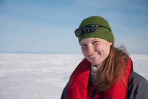
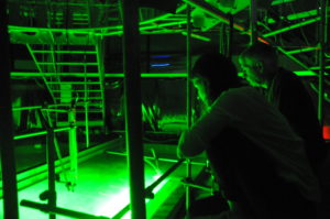
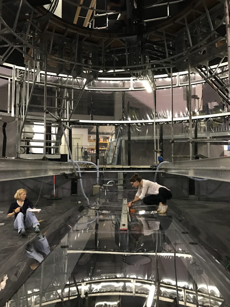
When we want to show people images of our model experiments in a tank, people often imagine that they will be shown cute little miniature landscapes, looking much like the ones you see for really fancy model train setups. And then they are hugely disappointed when they see pictures like the one below and we tell them that yes! that’s our Antarctica that Nadine is climbing on, while Elin is sitting in the Southern Ocean.

The kind of experiment everybody hopes to see could, according to Faller (1981), be classified as a simulation: representing the natural world in miniature, including every detail. Data from those experiments — since they would in theory be realistic representations of the real world — could be used to fill in missing data from the real world in regions that are hard to get real data from, like for example the Southern Ocean. However, since those experiments are designed to represent the complexity of the real world, interpretation of the experiments is as complex as it is to interpret data from the real world: There are so many processes involved that it is hard to isolate effects of individual processes.

The kind of experiments we are doing would be classified as abstractions. Faller describes this kind of experiment as similar to abstract art: Only the main features, or better: the artist’s interpretation of the main features, are reproduced and everything else is omitted. That makes the art difficult to understand for anyone who isn’t well versed in abstract art, but for the experts it is obvious what the point is.

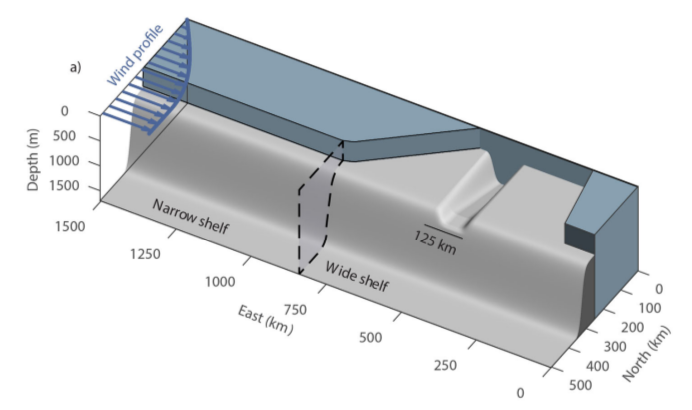
In case of our experiments that means that we have all the relevant features, or better: our interpretation of what we believe to be relevant features, of Antarctica present in the tank: the parts of topography that we think have an influence on how the current should behave, i.e. a V-shaped canyon, a source that supplies water of the correct properties into the ambient “ocean” water, an ice shelf. And when that ice shelf is tilted, we feel like our experiments are already becoming pretty realistic!

These abstractions are the kinds of experiments in which you can, because they are relatively simple, develop new theories when new features of the circulation emerge that you then have to rationalize and include in your theories after the fact.

We have actually also done another type of experiment, a verification. I wrote about it in this post: we tilted the ice shelf because this is a case for which we actually knew from theory how our current should behave, in contrast to all the previous experiments where we didn’t actually know what to expect, and we were happy when we observed exactly what we expected based on theoretical considerations. So in this case the experiment wasn’t about discovering something new, but rather making sure that our understanding of theory and what goes on in the tank actually match.

Faller describes a last type of experiment: the extension. That is the kind of experiment that you could perform after a successful verification experiment: Pushing the boundaries of the theory. Does it still hold if the current introduced in the tank is very fast or very slow? If the water is very deep? If the slope of the ice shelf is very large or small? Basically, every parameter could now be changed until we know for which cases the theory holds, and for which it does not.

So why am I writing all of this today? Faller’s (1981) article, before he goes on to describe the framework to think about geophysical fluid dynamics experiments that I mentioned above and which I find quite helpful to consider, starts with the sentence “No one believes a theory, except the theorist. Everyone believes an experiment — except the experimenter.” On this blog, our goal is to bring the two together and not make anyone believe either of them, but to show how both can work together to mutual benefit.

Faller, A. J. (1981). The origin and development of laboratory models and analogues of the ocean circulation. Evolution of Physical Oceanography, 462-479.

Idealised modeling in a different way

Written by Svenja Ryan

After our excursion to ‘real’ Antarctica, we are back in the idealised world. Hopefully you all have followed the blog and have seen how our continental shelf has been constructed and the source for our current has been tested. The same thing has been done by one of our colleagues, Kjersti, on the computer to then run it with a regional ocean model. In Figure 1 you can see the similarity of the set-up that she created to the one in our tank. The advantages of here experiments are that she can add a wind-forcing of any strength at the surface and can also change the surface temperature and salinity fields to mimic the seasonally varying effect of sea ice. Furthermore, she located a dense source at the end of the trough representing the dense water outflow.

Idealized model configuration from Daae et al., 2017. The model domain consist of a narrow and a wide shelf region with a trough cross-cutting the wide shelf. The set-up is based on the shelf on front of the Filchner Ice shelf. The blue arrows indicate the imposed zonal wind profile.

In her recent publication (Daae et al., 2017) she uses this model to study the sensitivity of the warm deep water entering a continental shelf with a coastal trough to the magnitude of wind stress, the shelf salinity and the upper-layer hydrography. She finds that stronger along-slope winds create a stronger slope current which is also shifted toward shallower isobaths, causing a stronger interaction of the flow with the trough. At low wind speeds the core of the current is located below the depth of the sill and is not affected. The southward transport of warm deep water increases for a denser outflow and higher salinities on the shelf. This effect is stronger for weak winds compared to strong winds, potentially because a strong barotropic flow passing the mouth of the trough will create less baroclinic instabilities.

They find that the warm deep water mainly accesses the shelf when no work against the buoyancy force has to be done. This is the case when dense water on the shelf connects the density surfaces between the shelf and off-shelf water masses. Furthermore, more warm water is found on the shelf in summer, when a fresh surface layer is present due to the sea ice melting. It induces a shallow eddy overturning cell that acts to flatten the isopycals, hence providing easier access to the shelf.

You see that you can sort of play god with these models, but you actually have to be very careful to choose all your parameters correctly and in a way that they representable for the processes in nature. Handled with care, models provide another important tool for understanding the climate system and individual processes.

Daae, K. B., Hattermann, T., Darelius, E., & Fer, I. (2017). On the effect of topography and wind on warm water inflow – An idealized study of the southern Weddell Sea continental shelf system. Journal of Geophysical Research : Oceans, 122, 2017-2033. http://doi.org/10.1002/2016JC012541

A bit more about real Antarctica

Written by Svenja Ryan

We have already written about the article of Elin, where she shows that for the first time pulses of warm water have been measured in the vicinity of the ice front. This means that under certain conditions the warm water, can travel several hundred kilometers south along the eastern side of the Filchner depression, i.e. our trough. Of course everyone wants to know whether the trough provides a permanent pathway to the south for the warm water, which would be a big threat to the Filchner Ronne Ice Shelf.

We will come back to this problem in a little while but first have to explain something that we call ‘Antarctic Slope Front’.  I think most of you are familiar with weather fronts, where for example cold and warm air meet. The same things exist in the ocean, when warm and cold or light and dense water masses encounter each other. This exactly is the cast almost all the way around Antarctica where fresh and cold water is found on the continental shelf and warm water (CDW/WDW) flows along the continental slope. The resulting front is the Antarctic Slope Front (ASF) as show in Figure 1. The depth of this front determines whether the deeper warm water can access the continental shelf or not. During our experiments we will also introduce a density difference at some point by have saline water in the tank and a fresh source.

Figure 1: A cross-section of the land ice – shelf ice – ocean system, showing the cold water on the continental shelf and below the ice shelf and the warm water situated just off the coast. (Illustration: Ole Anders Nøst, Norwegian Polar Institute).

Several mechanisms can influence the ASF such as the wind and the upper-layer hydrography, both having a strong seasonal cycle. Therefore, it is no surprise that the ASF depth also varies seasonally and it has been shown by various authors, that it is shallower in summer, favoring on-shelf flow of warm water and deeper in winter, reducing the access for warm deep water.

Figure 2: Station plot from Ryan et al., 2017 with the warm coastal current in grey and warm intrusions onto the continental shelf in dashed grey. Blue and red arrows show pathways of the cold water emerging from underneath the ice shelf. Coloured dots represent hydrographic stations and the other symbols moorings.

So, now we know that there might not be warm water available at the shelf break to flow toward the ice front at any time. Another important factor is whether the circulation on the continental shelf would transport the warm water toward the ice front all year around. Hence, we took the German ice breaker RV Polarstern and went to the Filchner region to put some more instruments in the water and I analyse the data in my recent publication (Ryan et al., 2017).  The map in Figure 2 should sort of look familiar to you now as it similar to the one in a previous article. You can see the coast to the right, then the continental shelf (Eastern Shelf) that opens up and the trough cross-cutting the shelf toward the Filchner Ice Shelf. We put moorings, i.e. a long upright floating lines with instruments at different depths, where the three red stars are on the map and left them there for two years. It is the eastern flank of the trough, where the warm water (dashed gray arrow) was observed to flow south adjacent to the northward flowing cold water, called Ice Shelf Water, emerging from underneath the ice shelf (blue arrow). You can see in Figure 3 how this looks like in a temperature section and where we took our measurements. You might wonder, why we did not put instruments shallower than 300m. If we did, we would risk these instruments to be ripped off by ice bergs, and there are plenty of them around. We found that there is only a certain period in summer-autumn, where we detect southward flowing warm water at our moorings. In winter, the water column becomes very cold and uniform with temperatures close to the surface freezing point and there is no southward flow anymore. So for now it seems like there is no permanent pathway for the warm water toward the Filchner Ice Front. However, in a warming climate the conditions on the continental shelf in winter could change, with warmer atmospheric temperatures and reduced sea ice production. The latter, could also reduce the production of ISW which is currently filling the whole trough and is sort of ‘blocking’ the warm water from entering the centre of the trough.

Figure 3: A temperature sections across the eastern flank of the trough (see black ellipse on Map for location) and the setup of the moorings.

Of course we do not have winds, ice etc. in our tank experiments but there is still so much more to be understood on how the warm water can be transported on the shelf and how for example the ASF changes in the vicinity of a coastal trough. Most measurements or time series are too short or too scattered in order to really understand fundamental processes and mechanisms, this is where a big rotating tank can help us!

Ryan, S., Hattermann, T., Darelius, E., & Schröder, M. (2017). Seasonal Cycle of Hydrography on the Eastern Shelf of the Filchner Trough, Weddell Sea, Antarctica. Journal Geophysical Research – Oceans. http://doi.org/10.1002/2017JC012916