Month: September 2017

A very convenient way to describe a flow system is by looking at its Froude number. The Froude number gives the ratio between the speed a fluid is moving at, and the phase velocity of waves travelling on that fluid. And if we want to represent some real world situation at a smaller scale in a tank, we need to have the same Froude numbers in the same regions of the flow.

For a very strong example of where a Froude number helps you to describe a flow, look at the picture below: We use a hose to fill a tank. The water shoots away from the point of impact, flowing so much faster than waves can travel that the surface there is flat. This means that the Froude number, defined as flow velocity devided by phase velocity, is larger than 1 close to the point of impact.

At some point away from the point of impact, you see the flow changing quite drastically: the water level is a lot higher all of a sudden, and you see waves and other disturbances on it. This is where the phase velocity of waves becomes faster than the flow velocity, so disturbances don’t just get flushed away with the flow, but can actually exist and propagate whichever way they want. That’s where the Froude number changes from larger than 1 to smaller than 1, in what is called a hydraulic jump. This line is marked in red below, where waves are trapped and you see a marked jump in surface height. Do you see how useful the Froude number is to describe the two regimes on either side of the hydraulic jump?

Obviously, this is a very extreme example. But you also see them out in nature everywhere. Can you spot some in the picture below?

But still, all those examples are a little more drastic than what we would imagine is happening in the ocean. But there is one little detail that we didn’t talk about yet: Until now we have looked at Froude numbers and waves at the surface of whatever water we looked at. But the same thing can also happen inside the water, if there is a density stratification and we look at waves on the interface between water of different densities. Waves running on a density interface, however, move much more slowly than those on a free surface. If you are interested, you can have a look at that phenomenon here. But with waves running a lot slower, it’s easy to imagine that there are places in the ocean where the currents are actually moving faster than the waves on a density interface, isn’t it?

For an example of the explanatory power of the Froude number, you see a tank experiment we did a couple of years ago with Rolf Käse and Martin Vogt (link). There is actually a little too much going on in that tank for our purposes right now, but the ridge on the right can be interpreted as, for example, the Greenland-Scotland-Ridge, making the blue reservoir the deep waters of the Nordic Seas, and the blue water spilling over the ridge into the clear water the Denmark Strait Overflow. And in the tank you see that there is a laminar flow directly on top of the ridge and a little way down. And then, all of a sudden, the overflow plume starts mixing with the surrounding water in a turbulent flow. And the point in between those is the hydraulic jump, where the Froude number changes from below 1 to above 1.

Nifty thing, this Froude number, isn’t it? And I hope you’ll start spotting hydraulic jumps every time you do the dishes or wash your hands now! 🙂

—

All pictures in this post are taken from my blog “Adventures in Oceanography and Teaching“. Check it out if you like this kind of stuff — I do! 🙂

When we come back from research cruises, one of the things that surprises people back home is how much time it takes to take measurements. And that’s for two reasons: Because the distances we have to travel to reach the area we are interested in are typically very large. And then because the ocean is also very deep.

People usually find it hard to imagine that it can easily take hours for an instrument, hanging on a wire from the ship, to go down all the way to the sea floor and then come back up to the ship again. A typical speed the winch is run at is 1 m/s. That means that for a typical ocean depth of 4 km, it takes 66 minutes for the instrument to go down, and then another hour to be brought back up to the ship. And then we haven’t even stopped the winch on the way up, which we usually do each time we want to take a water sample. So yes, the ocean is very deep!

And yet, it is not deep. At least not compared to its horizontal extent. The fastest crossing of the Atlantic, some 5000km, took something like 3 days and 10 hours. And according to a quick google search, a container ship typically takes 10 to 20 days these days. So there is a lot of water between continents! And it is really difficult to imagine how large the oceans really are.

One way to describe the extent of the ocean is to use the L/H aspect ratio. It is just the ratio between a typical length (L), and a typical depth (H). A typical east-west length in the Atlantic are our 5000 km used above, and a typical depth are 4 km. This gives us an aspect ratio L/H of 5000/4 which is 1250. That is actually a really large aspect ratio — the horizontal length scales are a lot wider than the vertical ones.

Now think about the kind of tank experiments we typically do. Here is a picture of a very simple Denmark Strait overflow experiment (more on that experiment here). You see the tank in the foreground, and a sketch of the same situation on the wall in the background. What you notice both for the experiment and the depiction is that in both cases the horizontal length scale is only about twice as much as the vertical one, leading to a L/H of 2.

This L/H of 2, however, is supposed to represent a situation that in the real world has a horizontal scale of maybe 1000 km and a vertical one of maybe 1 km, which leads to a L/H of 1000. So you see that the way we typically depict sections through the ocean is very distorted from what they would look like if they were geometrically similar, meaning that they had the same L/H ratio, which means that they could be transformed into the real world just by uniformly stretching or shrinking.

Below I have sketched a couple of duck ponds. The one on the left (with an aspect ratio L/H of 1) is geometrically shrunk below: Even though L and H become smaller, they do so at the same rate: their ratio stays the same. However going along the top row of duck ponds, the aspect ratio increases: While L stays the same, H shrinks. This means that the different ponds along the top of the picture are not geometrically similar. However, the one on the top right is geometrically similar to the one in the bottom right again (both have an L/H of 6). Does this make sense?

So in case you were wondering about why we need a tank that has 13 meters diameter — maybe now you see that it allows us to maintain geometric similarity a lot better than a smaller tank would, at least when we want to have water depths that are large enough that allow us to neglect surface tension effects and all that nasty stuff.

More on how Elin actually designed the experiments soon! 🙂

When talking about oceanographic tank experiments that are designed to show features of the real ocean, many people hope for tiny model oceans in a tank, analogous to the landscapes in model train sets. Except even tinier (and cuter), of course, because the ocean is still pretty big and needs to fit in the tank.

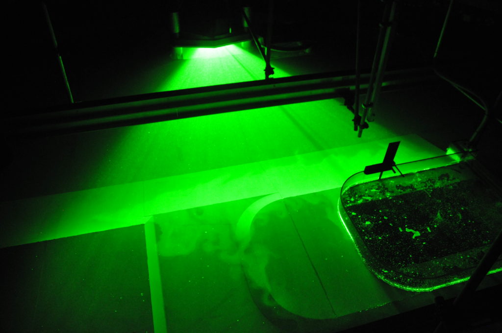
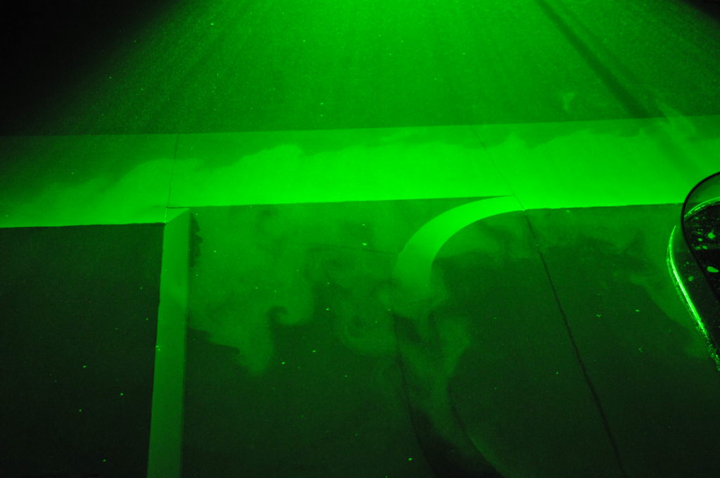
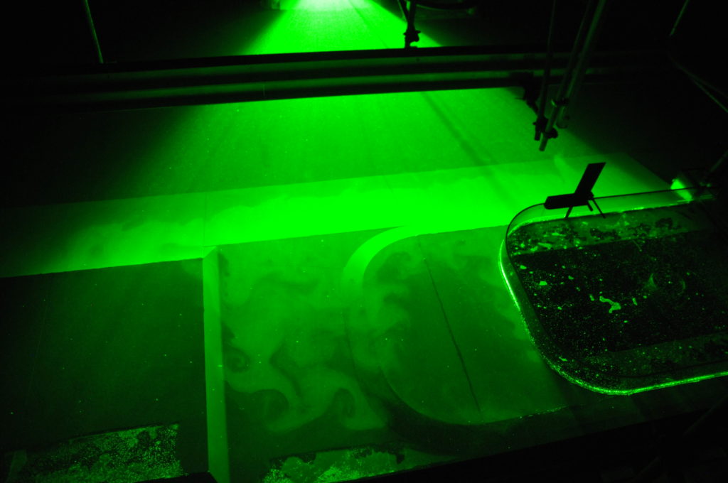
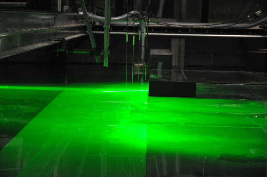
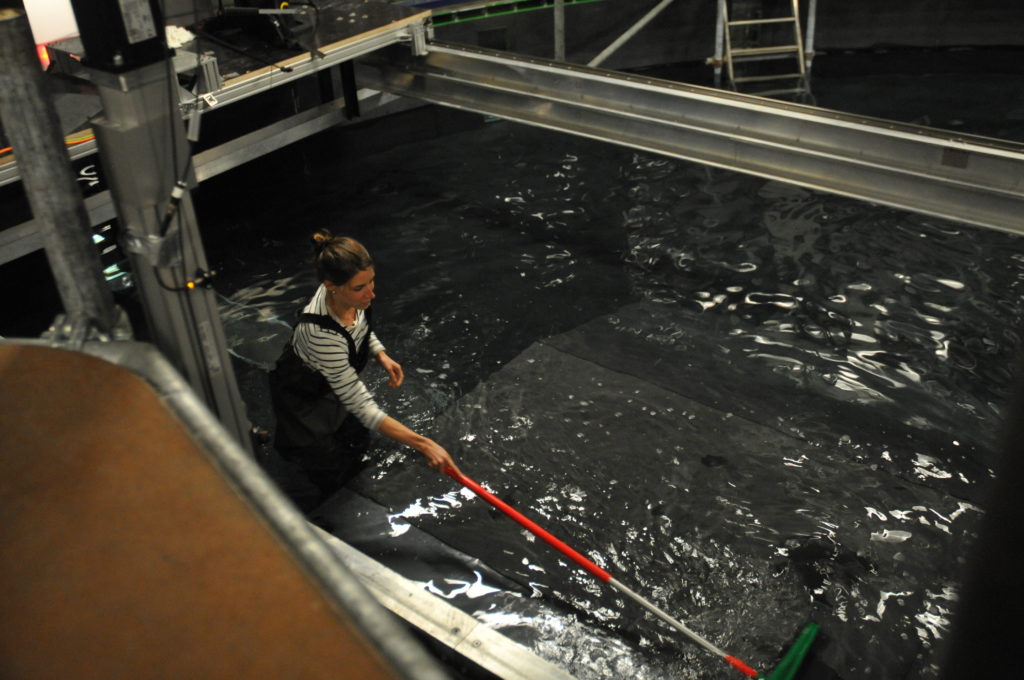
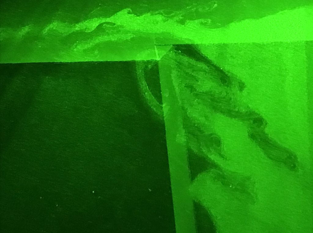
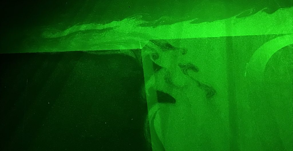
What people hardly ever consider, though, is that purely geometrical downscaling cannot work. Consider, for example, surface tension. Is that an important effect when looking at tides in the North Sea? Probably not. If your North Sea was scaled down to a 1 liter beaker, though, would you be able to see the concave surface? You bet. On the other hand, do you expect to see Meddies when running outflow experiments like this one? And even if you saw double diffusion happening in that experiment, would the scales be on scale to those of the real ocean? Obviously not. So clearly, there is a limit of scalability somewhere, and it is possible to determine where that limit is – with which parameters reality and a model behave similarly.

Similarity is achieved when the model conditions fulfill the three different types of similarity:

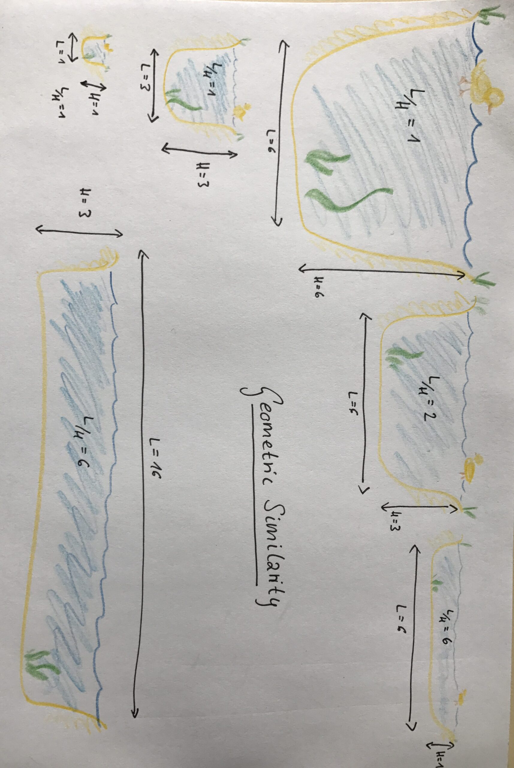
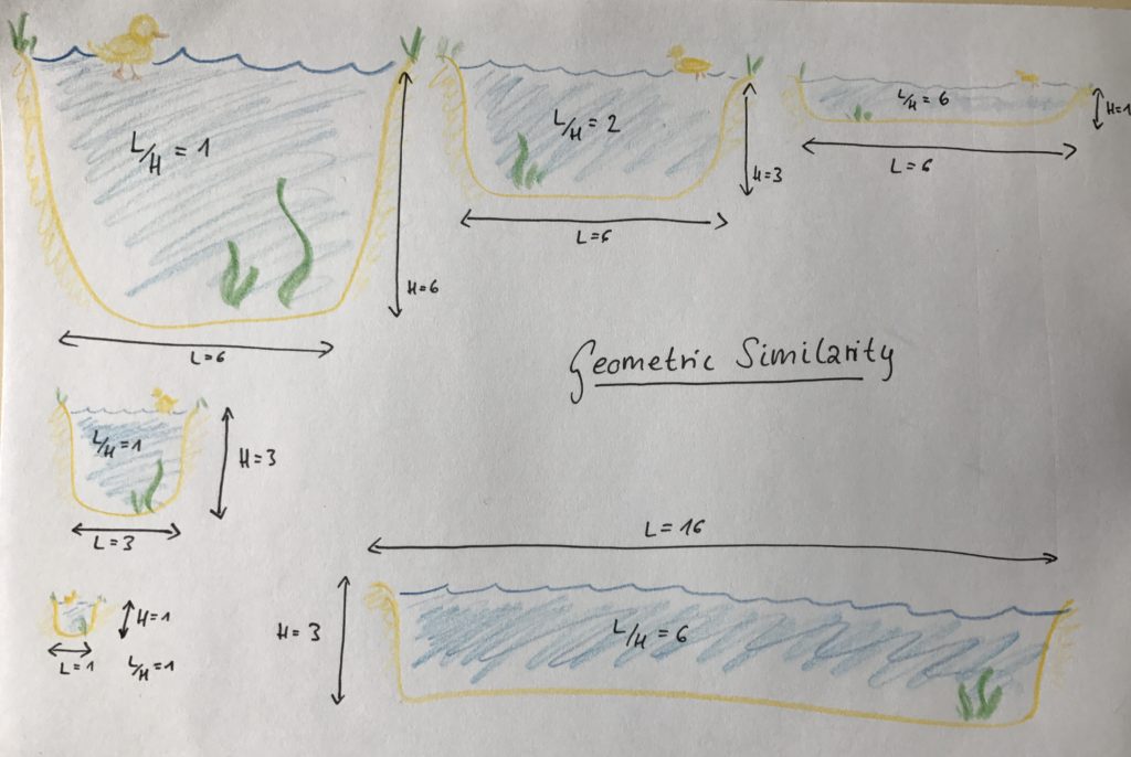
Geometrical similarity
Objects are called geometrically similar, if one object can be constructed from the other by uniformly scaling it (either shrinking or enlarging). In case of tank experiments, geometrical similarity has to be met for all parts of the experiment, i.e. the scaling factor from real structures/ships/basins/… to model structures/ships/basins/… has to be the same for all elements involved in a specific experiment. This also holds for other parameters like, for example, the elastic deformation of the model.

Kinematic similarity
Velocities are called similar if x, y and z velocity components in the model have the same ratio to each other as in the real application. This means that streamlines in the model and in the real case must be similar.

Dynamic similarity
If both geometrical similarity and kinematic similarity are given, dynamic similarity is achieved. This means that the ratio between different forces in the model is the same as the ratio between different scales in the real application. Forces that are of importance here are for example gravitational forces, surface forces, elastic forces, viscous forces and inertia forces.

Dimensionless numbers can be used to describe systems and check if the three similarities described above are met. In the case of the experiments we talk about here, the Froude number and the Reynolds number are the most important dimensionless numbers. We will talk about each of those individually in future posts, but in a nutshell:

The Froude number is the ratio between inertia and gravity. If model and real world application have the same Froude number, it is ensured that gravitational forces are correctly scaled.

The Reynolds number is the ratio between inertia and viscous forces. If model and real world application have the same Reynolds number, it is ensured that viscous forces are correctly scaled.

To obtain equality of Froude number and Reynolds number for a model with the scale 1:10, the kinematic viscosity of the fluid used to simulate water in the model has to be 3.5×10^-8m²/s, several orders of magnitude less than that of water, which is on the order of 1×10^-6m²/s.

There are a couple of other dimensionless numbers that can be relevant in other contexts than the kind of tank experiments we are doing here, like for example the Mach number (Ratio between inertia and elastic fluid forces; in our case not very important because the elasticity of water is very small) or the Weber number (the ration between inertia and surface tension forces). In hydrodynamic modeling in shipbuilding, the inclusion of cavitation is also important: The production and immediate destruction of small bubbles when water is subjected to rapid pressure changes, like for example at the propeller of a ship.

It is often impossible to achieve similarity in the strict sense in a model experiment. The further away from similarity the model is relative to the real worlds, the more difficult model results are to interpret with respect to what can be expected in the real world, and the more caution is needed when similar behavior is assumed despite the conditions for it not being met.

This is however not a problem: Tank experiments are still a great way of gaining insights into the physics of the ocean. One just has to design an experiment specifically for the one process one wants to observe, and keep in mind the limitations of each experimental setup as to not draw conclusions about other processes that might not be adequately represented.

So much for today — we will talk about some of the dimensionless numbers mentioned in this post over the next weeks, but I have tried to come up with good examples and keep the theory to a minimum! 🙂