We’re in Nature!

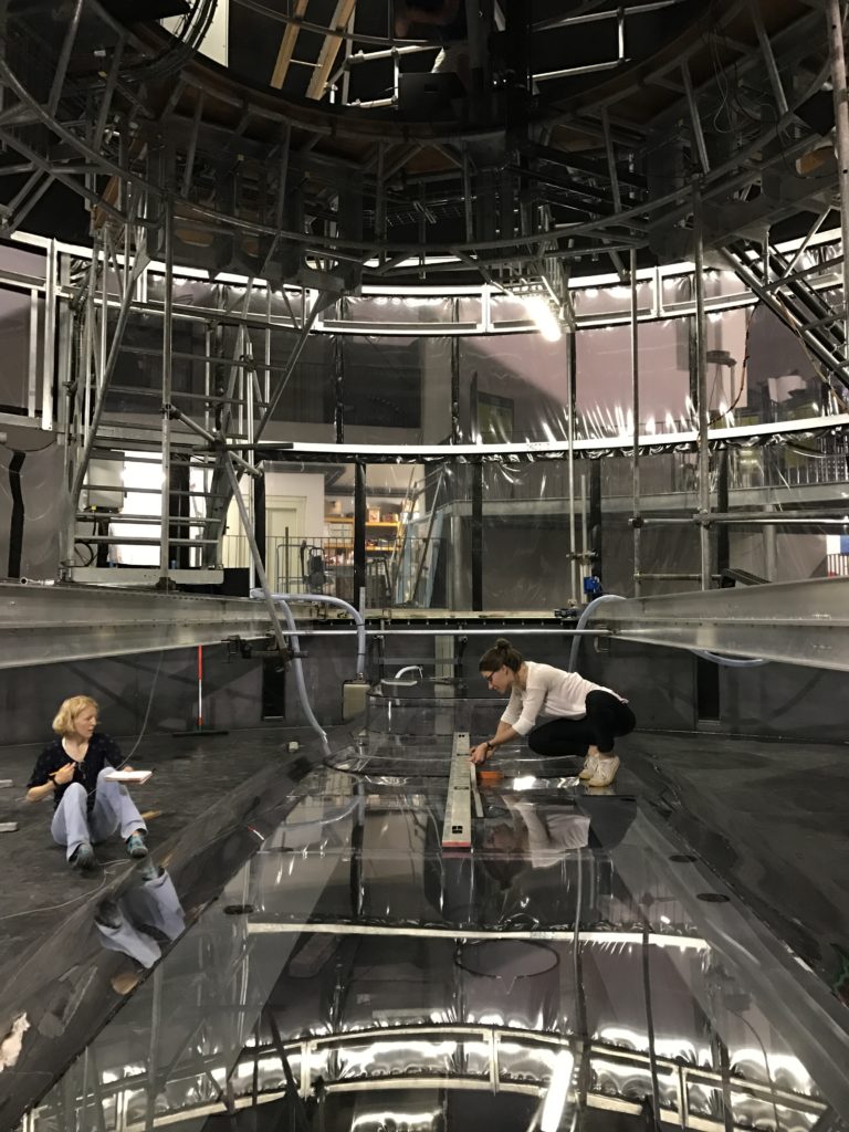
I remember vivid discussions with Anna over a loaf of freshly baked bread from our new bread machine. We were in the Southern ocean, somewhere in between New Zealand and the Getz Ice shelf in the Amundsen Sea on board the Korean icebreaker Araon and we talked about the moorings we were about to deploy, the proposal we have started writing, the experiments we wanted to run – but most of all we talked about what actually happens when ocean currents meet an ice shelf front. That was four years ago – and I’m super excited to see that a few days the results of those discussions (and a good deal of work on board Araon, on and around the rotating Coriolis platform in Grenoble and in numerous offices around the world) were published in Nature! Ice front blocking of ocean hear transport to an Antarctic ice shelf by A. Wåhlin, N. Steiger, E. Darelius, K. M. Assmann, M. S. Glessmer, H. K. Ha, L. Herraiz-Borreguero, C. Heuze, A. Jenkins, T.W. Kim, A. K. Mazur, J. Sommeria and S. Viboud – in Nature! (For those of you who are not into peer reviewed litterature and scientific publishing – this is probably scientific equivalent to an Olympic gold medal!)

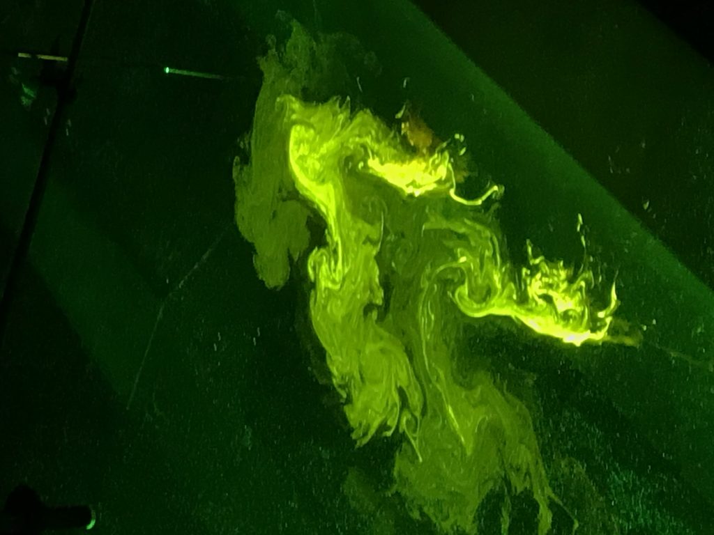
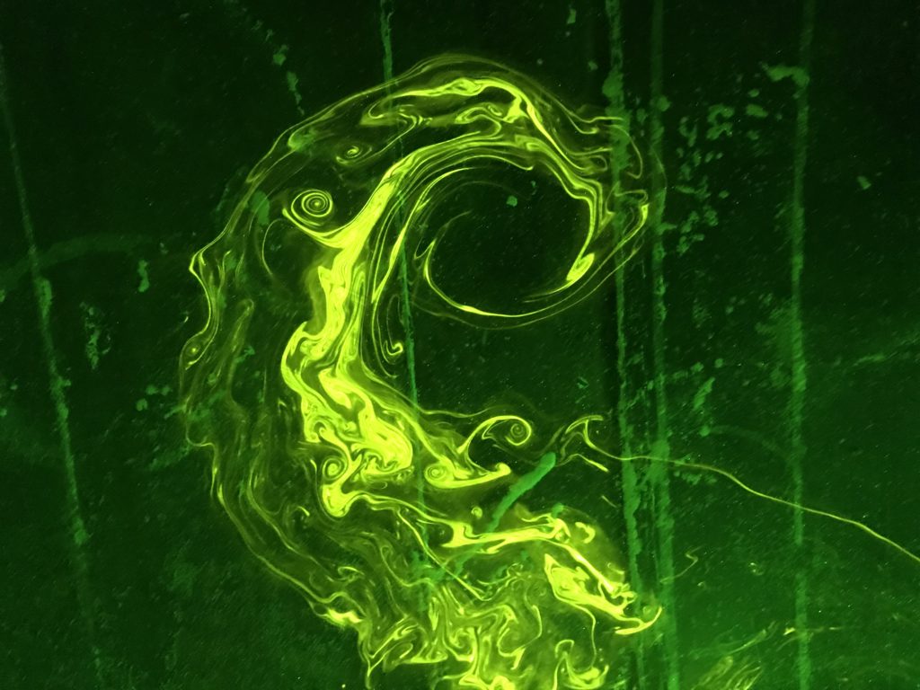
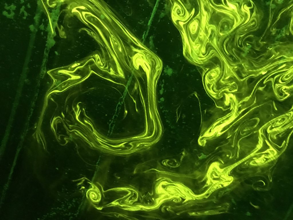
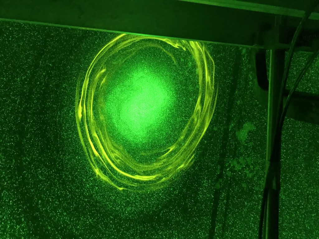
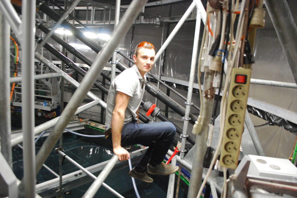
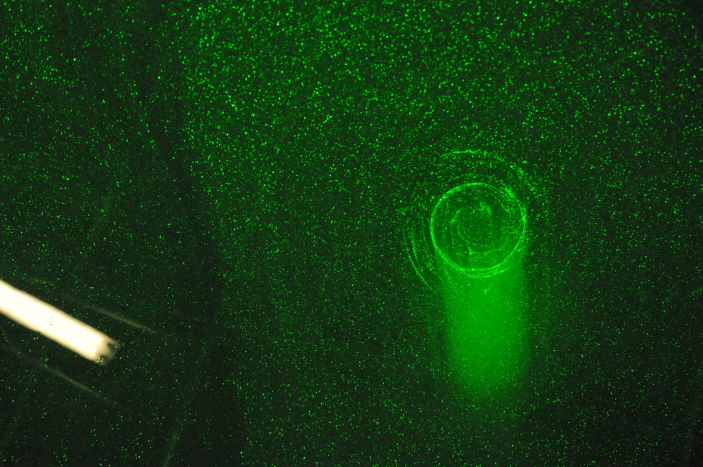
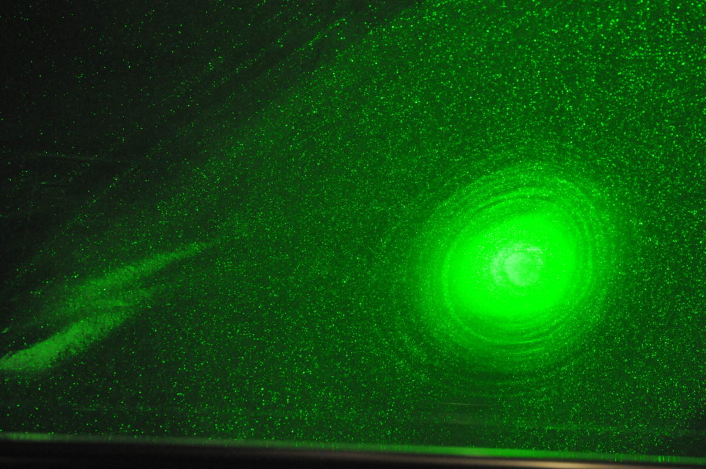
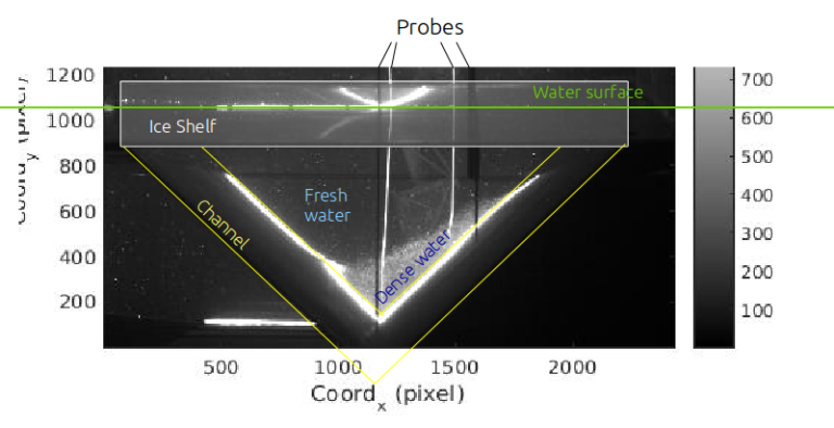
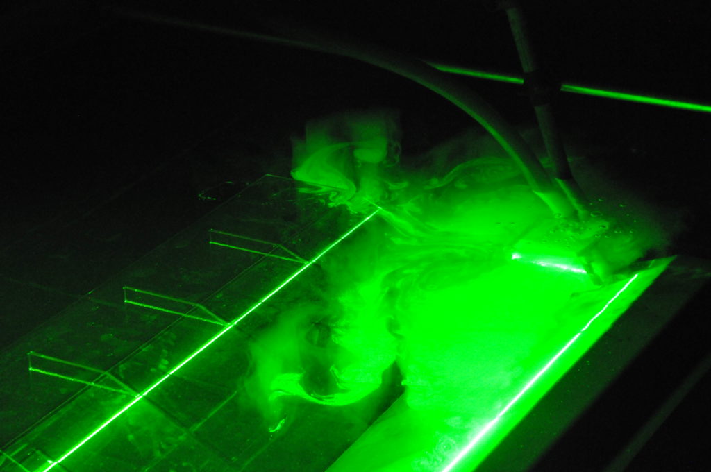
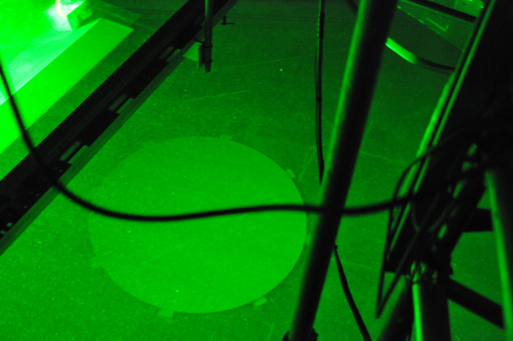
So what did we find out – well, to make a long story short – we oceanographers talk about two types of currents. They are both driven by pressure gradients – but for what we call barotropic currents, the pressure gradient is caused by differences in sea level (i.e. in how much water there is) while for baroclinic currents, the pressure gradient is caused by differences in density (i.e. how heavy the water is).  The barotropic current is depth independent – this means that the current is equally strong from the surface down to the bottom, while the baroclinic current changes in strength (and potentially in direction) with depth. Our observations showed that the currents bringing heat towards the Getz ice shelf had both a barotropic and a baroclininc (bottom intensified) part. The barotropic part was the stronger one and the one carrying the majority of the heat. But when the current reached the ice shelf front (Anna was brave enough to deploy a mooring only 700m from the ice shelf front)  – the strong barotropic current had to turn, and only the weaker baroclinic current was able to enter the ice shelf cavity. The experiments at the rotating table showed the same thing – barotropic currents turned at the front, while baroclinic currents could enter.

Experiments at the Coriolis platform in Grenoble – a 13 – m large combination of a swimming pool and a merry-go-round!

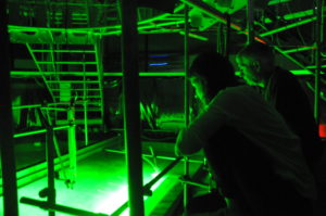
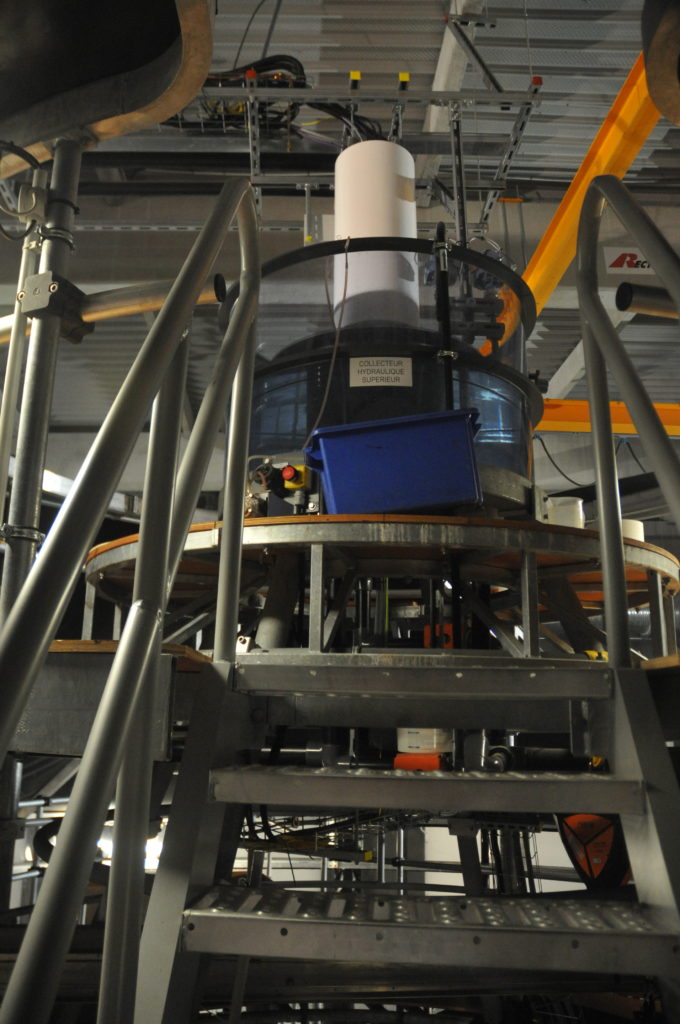
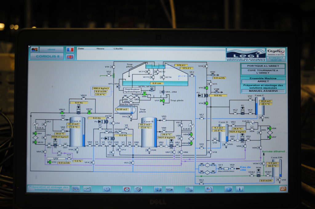
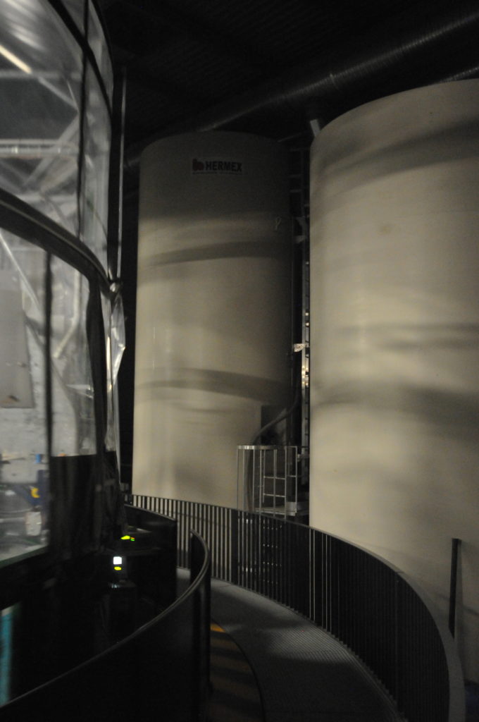
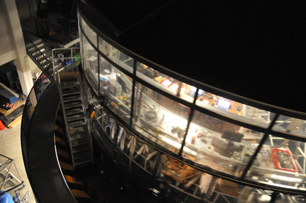
You can read more about what we did in the Coriolis lab here, and about when Karen recovered the moorings here

Scrolling back memory lane: Reminiscing of rotation

Hei, remember we were in Grenoble and did exciting experiments on the 13-m-dimeter pool on a merry-go-round only last autumn? Feels like a long time ago already. But here are two ways for you to scroll back memory lane:

  1. Check out the new way we’ve created to access to Elin & her team’s previous adventures on our “previous adventures” page. Did you know we have posts in English, Norwegian and Swedish, addressing audiences from primary school kids, over high school pupils, to teachers, our fellow oceanographers and friends and family? Quite impressive how much Elin has written over the years, and fascinating to read, too! And also check out her ongoing adventures like the student cruise to Bjørnafjorden!

2. Read the award-winning* poem below which I just found somewhere in my files. Yes, we did feel not quiiiite well when we were working on the platform at high rotation rates, but we still loved the whole experience, every minute of it! 🙂

*Yes, this poem really won an award in a competition run by @IAmSciComm on Twitter back in October. And here is the awesome bag and sea horse card we won 🙂

Mesmerizing flow patterns and sad goodbyes

Written by Anna Wåhlin

It is the final day of experiments here at the Coriolis platform. The apartment is emptied of personal belongings, bicycles are being returned, goodbyes are stretched out. The lasers will soon be dark, the platform will grind to a halt and the tank will be emptied. It has been a fantastic time! I am amazed at what we have accomplished together during these weeks – answers to some of the most basic questions that are currently asked about the future for the Antarctic ice sheet.

Figure 2a-d: More mesmerizing flow patterns

The last days have been spent re-running some of the experiments that needed an extra quality-check, and we finished the very last one only an hour ago. Next week I will stay behind alone to try to get some nice photographs of the flow for our future publications. In order to prepare for that we were testing some different dyes. Red dye absorbs the light of the laser efficiently and gives a dark shadow on the images. Our all time favorite is Rhodamin – it is a fluorescent dye that produces its own light if you shine on it with green laser. We spent a good hour simply staring at the eddies and flow, mesmerized by the motion and flowing patterns. A very fine ending to the week! And a suitable finale to the time we have spent here on the rotating platform.

Video: Visualization of a beautiful barotropic eddy created outside the channel. It stayed like this for a good hour. You can see the barotropic structure since it moves in unison on the surface and below the surface, in a nearly perfect two-dimensional motion.

Introducing: Thomas Valran and Samuel Viboud

We have presented all the scientists that are involved in the project, but still haven’t introduced the two most important people: Samuel and Thomas without whom we would not have been able to conduct the experiments.

Today, part 2: Samuel Viboud, for Thomas see here.

Samuel is an engineer in experimental techniques on large instruments and has been working at LEGI since 2001, when it was still at another place in Grenoble where Elin, Anna and Adrian conducted experiments about 10 years ago. To be in charge of the rebuild of the Coriolis platform was the most exciting event for him. Samuel is the technical director of the Coriolis platform and the head of the mechanical department at LEGI. Thanks to his creativity, technical know-how and sense for innovation, he received the well-deserved “Médailles de cristal” from CRNS in 2015.
About his personal life he says:
“Coming from a winemaker family who cultivates the grape varietal: “Mondeuse”, I live in the village of Apremont in Savoie, and do not hesitate to spend my time with work such as harvesting and bottling. In my personal life that I share with my wife and my 2 children, the exchange, the attention and the mutual support are daily. Concerning leisure, I am passionate about sport and particularly about road cycling. I regularly climb the mountain passes of the region and commute 100km to work by bike. The mountains are also my playground especially in winter, with ski touring that I like to share with my friends. What characterizes me in the end in life as at work are the essential values such as: sharing, conviviality and family.”


Introducing: Thomas Valran and Samuel Viboud

We have presented all the scientists that are involved in the project, but still haven’t introduced the two most important people: Samuel and Thomas without whom we would not have been able to conduct the experiments.

Today, part 1: Thomas Valran.
Part 2 to follow on Monday

Thomas is an engineer at the Coriolis platform and has been working for LEGI since March 2016. During his diploma in industrial engineering at the “Ecole nationale supérieure des Mines de Saint-Etienne” he worked as apprentice engineer for Schneider Electric. At the Coriolis platform, the most exciting part for him is to work for many different projects that never make the job boring. Due to his experience in climbing he moves on the supports of the platform very gently despite the high rotation speed. In his spare time, Thomas likes to go on road trips with his motorcycle or help at his parent’s farm where he grew up and where there are about 100 cows to take care of.

We discovered a new galaxy! Or at least a very pretty vortex

When we move our wall back and forth, we create very strong wing tip vortices that persist for quite a long time.

Above, you see the vortex, lit by a laser sheet close to the surface. You can see the whole column rotating as one, that bright smudge below the swirl is the lower part of the column. There are so many of our neutrally buoyant particles in there that the column looks bright even though it isn’t directly lit by the laser.

And in the picture above, you see those bright smudges on the left of the picture? That’s particles that the vortex hoovered up and then dumped in its path, pretty much like a hurricane would.

And that’s what it looks like as a gif:

How salt changes the current

Until the beginning of the week we had only conducted barotropic experiments. This means that we induced fresh water into fresh water. How boring, you may thing… Well, although these experiments were very interesting, you are probably right because this setup doesn’t quite correspond to reality. At the coast of Antarctica, dense water is on one side produced by the growth of sea ice and on the other side origins from deep water that spills over the coast onto the continental shelf. Because the continental shelf slopes down towards the ice shelf, the dense water reaches towards the ice shelf. Our aim is to find out how the water behaves as it reaches the ice shelf front.

To reproduce this dense water flow, we inject salt enriched water into the channel. This relatively dense water approaches the ice shelf front along the left channel slope. To see a clear boundary between the dense and the fresh water, only a density difference of 1 kg/m3 is needed. The density difference increases the velocity of the current a lot, so that the experiments last much shorter. While the barotropic current was mainly blocked by the ice shelf front, the baroclinic current can freely enter the cavity beneath the ice shelf, as the dense water is largely decoupled from the freshwater. Because the fresh water layer above the dense current is barotropic, the previous experiments were of big interest as well to see how the upper layer behaves as the current reaches the ice shelf front.

On the cross section through the channel, the dense water separates clearly from the freshwater. It flows parallel to the slope to its left. Because we built a wall at the end of the channel (see our previous post: https://elindarelius.no/2017/10/20/closing-off-our-channel-at-the-ice-shelf-end-to-avoid-unrealistic-outflow/), the channel fills up quickly with salt water, which we have to evacuate after each experiment.

The dense, saline water contains many particles and gets visible in the vertical laser sheet. It flows towards the ice shelf (=towards us) along the slope to its left side.

In the photo of the cross section, you can also see 4 probes sticking in the water that we use to measure the density close to the source and close to the ice shelf front. We can then calculate the velocity of the dense current and the mixing between the fresh water and dense water along the channel.

In this experiment, we injected a flow that is 1kg/m3 denser than the ambient water. During the scans, the vertical laser shows the position of the dense current and the 4 probes (2 in front of the ice shelf front, 2 in front of the vertical laser) measure the change in density with time.

Introducing: JB Sallée

Written by JB Sallée
JB Sallée is an oceanographer interested in the dynamics of the ocean and climate with active research efforts on the study of the Southern Ocean and Antarctica shelf circulation. His research mostly focuses on the observational connection between the ocean surface and the deep ocean interior, with particular emphasises ocean ice-sheet interaction as well as on heat, salt and anthropogenic carbon sequestration in the Southern Ocean. His research tackles questions from oceanic turbulence to large-scale ocean circulation, as well as on the impact of ocean physics on biology.

“No one believes a theory, except the theorist. Everyone believes an experiment — except the experimenter.”

Different types of experiments, and why we use such a weirdly-shaped “Antarctica” and are happy with it.

When we want to show people images of our model experiments in a tank, people often imagine that they will be shown cute little miniature landscapes, looking much like the ones you see for really fancy model train setups. And then they are hugely disappointed when they see pictures like the one below and we tell them that yes! that’s our Antarctica that Nadine is climbing on, while Elin is sitting in the Southern Ocean.

The kind of experiment everybody hopes to see could, according to Faller (1981), be classified as a simulation: representing the natural world in miniature, including every detail. Data from those experiments — since they would in theory be realistic representations of the real world — could be used to fill in missing data from the real world in regions that are hard to get real data from, like for example the Southern Ocean. However, since those experiments are designed to represent the complexity of the real world, interpretation of the experiments is as complex as it is to interpret data from the real world: There are so many processes involved that it is hard to isolate effects of individual processes.

The kind of experiments we are doing would be classified as abstractions. Faller describes this kind of experiment as similar to abstract art: Only the main features, or better: the artist’s interpretation of the main features, are reproduced and everything else is omitted. That makes the art difficult to understand for anyone who isn’t well versed in abstract art, but for the experts it is obvious what the point is.

In case of our experiments that means that we have all the relevant features, or better: our interpretation of what we believe to be relevant features, of Antarctica present in the tank: the parts of topography that we think have an influence on how the current should behave, i.e. a V-shaped canyon, a source that supplies water of the correct properties into the ambient “ocean” water, an ice shelf. And when that ice shelf is tilted, we feel like our experiments are already becoming pretty realistic!

These abstractions are the kinds of experiments in which you can, because they are relatively simple, develop new theories when new features of the circulation emerge that you then have to rationalize and include in your theories after the fact.

We have actually also done another type of experiment, a verification. I wrote about it in this post: we tilted the ice shelf because this is a case for which we actually knew from theory how our current should behave, in contrast to all the previous experiments where we didn’t actually know what to expect, and we were happy when we observed exactly what we expected based on theoretical considerations. So in this case the experiment wasn’t about discovering something new, but rather making sure that our understanding of theory and what goes on in the tank actually match.

Faller describes a last type of experiment: the extension. That is the kind of experiment that you could perform after a successful verification experiment: Pushing the boundaries of the theory. Does it still hold if the current introduced in the tank is very fast or very slow? If the water is very deep? If the slope of the ice shelf is very large or small? Basically, every parameter could now be changed until we know for which cases the theory holds, and for which it does not.

So why am I writing all of this today? Faller’s (1981) article, before he goes on to describe the framework to think about geophysical fluid dynamics experiments that I mentioned above and which I find quite helpful to consider, starts with the sentence “No one believes a theory, except the theorist. Everyone believes an experiment — except the experimenter.” On this blog, our goal is to bring the two together and not make anyone believe either of them, but to show how both can work together to mutual benefit.

Faller, A. J. (1981). The origin and development of laboratory models and analogues of the ocean circulation. Evolution of Physical Oceanography, 462-479.

How to make sure the properties of water in a tank experiment are *just right*

For all our experiments here on the rotating platform in Grenoble, we have had a source, introducing an artificial current into our water-filled tank. With flow rates between 15 l/min and 60 l/min, and experiments running for about half an hour, that is a lot of water that has to come out of the source!

Below, you see a picture of the source during an experiment, and you see there is a pipe going into it, through which water is being supplied.

That water is coming from the very top of the rotating platform. There is a smaller tank up there which you see on the picture below. This is the tank where the particles which we use to visualize the flow field get added, and water in this tank needs to have the exact density we want our inflow to have. Not easy since it is sitting some 10 meters above the tank, where the air temperature is higher…

In fact, it’s an extremely complex system of tanks everywhere on and around the rotating platform. Below you see a picture of the screen through which most of them are operated:

There are three huuuuge water tanks in which water is prepared. You might have seen them rotating past in some of our videos, or you see them below (on the left you see the rotating tank). This picture doesn’t do them any justice: They are enormous. They are higher than the tank, and the mini tank on top of it, and the whole tent around all of it, and they start from the very bottom of the room (so not the level that seems to be the floor in the picture below).

We got to climb on one of them, which gave us a really great view of the tank (or at least that’s what Nadine says, and what the picture looks like — I was too busy getting over my fear of heights combined with the dizziness of a long working day on the rotating platform to enjoy it much ;-)).

Nadine has described earlier about how for some experiments, we add salt to spice things up. In the first set of experiments, for some, the whole tank was filled with salt water. And for this set of experiments, we sometimes added a small amount of salt to adjust the density of the inflow. But this is how producing the salt water actually works: Salt arrives in big bags, stacked on pallets. The salt pellets are put into the bin you see in the picture below, and get hoovered up into one of the huge tanks, where they are dissolved in water to make a saturated salt solution. That solution is then diluted to whatever salt concentration is desired for a certain experiment.

To fill a whole tank with salt water with approximately oceanic salinity, we need all the salt shown in the picture above!

We are pretty lucky that Thomas and Samuel take care of all the saltwater-making for us. That would be a huge task if we had to do it ourselves, and we are already now not getting bored 😉

And, btw, if you are wondering about how we are getting rid of the dense, salty current that we inject into the fresh ambient water in between experiments: The dense water eventually sinks to the bottom of the tank, slowly filling it up underneath the fresher water. You might have noticed those UFO-shaped flat plates on the bottom of the tank that you see in the picture below. They cover the outlets through which the tank can be drained, such that now water from the very bottom of the tank can be pumped out without introducing a vertical component (which would suck water from higher levels, too).

Quite a lot of effort going on not only to prepare the water, but also to get rid of it again! 🙂