Idealised modeling in a different way

Written by Svenja Ryan

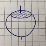
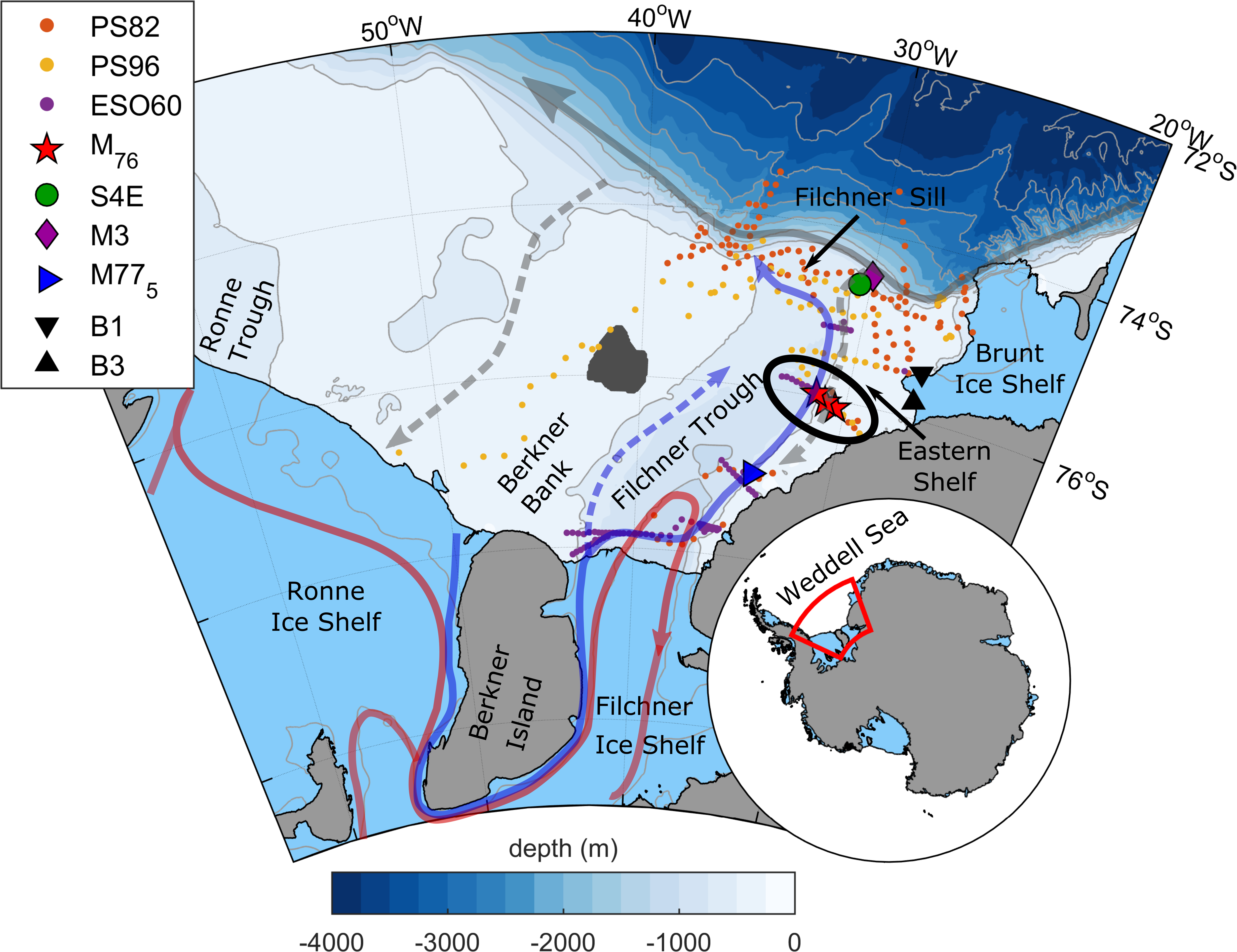
After our excursion to ‘real’ Antarctica, we are back in the idealised world. Hopefully you all have followed the blog and have seen how our continental shelf has been constructed and the source for our current has been tested. The same thing has been done by one of our colleagues, Kjersti, on the computer to then run it with a regional ocean model. In Figure 1 you can see the similarity of the set-up that she created to the one in our tank. The advantages of here experiments are that she can add a wind-forcing of any strength at the surface and can also change the surface temperature and salinity fields to mimic the seasonally varying effect of sea ice. Furthermore, she located a dense source at the end of the trough representing the dense water outflow.

Idealized model configuration from Daae et al., 2017. The model domain consist of a narrow and a wide shelf region with a trough cross-cutting the wide shelf. The set-up is based on the shelf on front of the Filchner Ice shelf. The blue arrows indicate the imposed zonal wind profile.

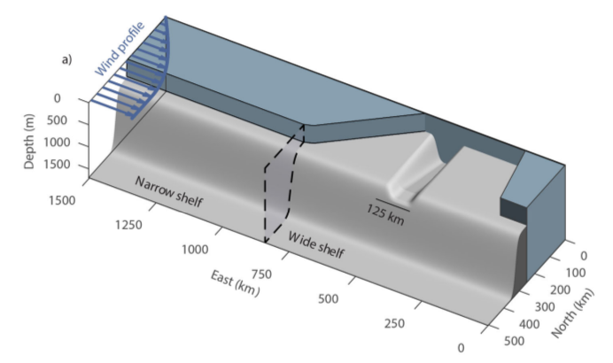
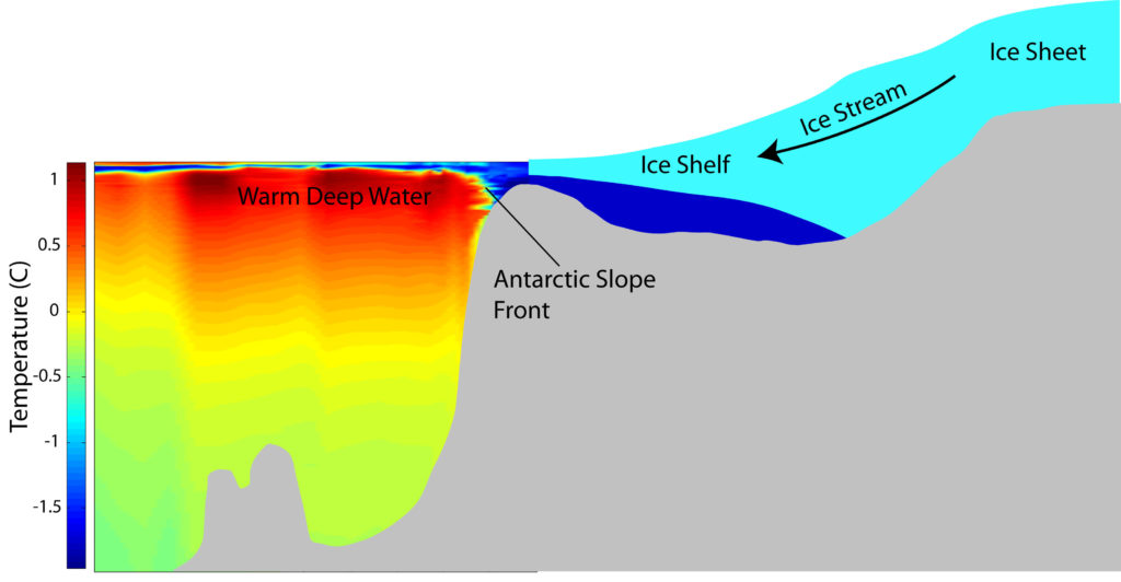
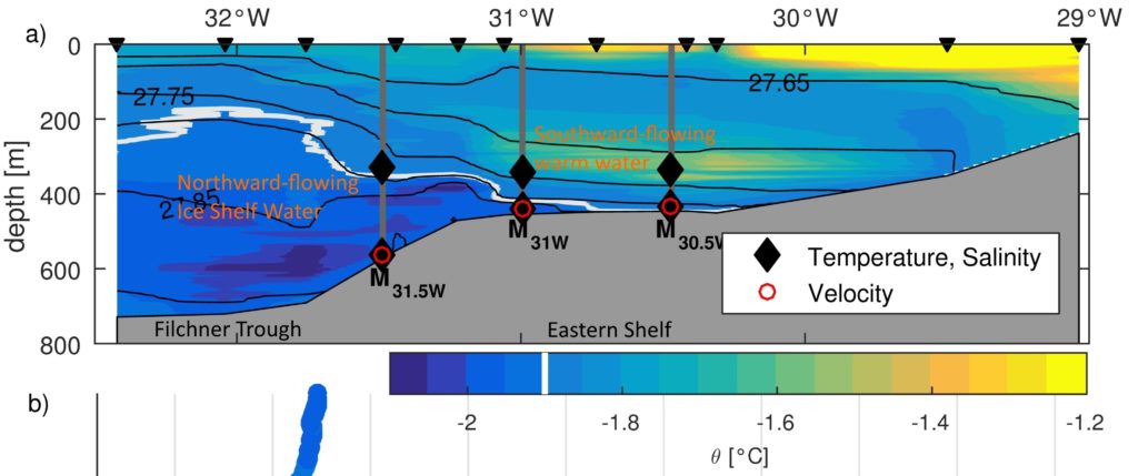
In her recent publication (Daae et al., 2017) she uses this model to study the sensitivity of the warm deep water entering a continental shelf with a coastal trough to the magnitude of wind stress, the shelf salinity and the upper-layer hydrography. She finds that stronger along-slope winds create a stronger slope current which is also shifted toward shallower isobaths, causing a stronger interaction of the flow with the trough. At low wind speeds the core of the current is located below the depth of the sill and is not affected. The southward transport of warm deep water increases for a denser outflow and higher salinities on the shelf. This effect is stronger for weak winds compared to strong winds, potentially because a strong barotropic flow passing the mouth of the trough will create less baroclinic instabilities.

They find that the warm deep water mainly accesses the shelf when no work against the buoyancy force has to be done. This is the case when dense water on the shelf connects the density surfaces between the shelf and off-shelf water masses. Furthermore, more warm water is found on the shelf in summer, when a fresh surface layer is present due to the sea ice melting. It induces a shallow eddy overturning cell that acts to flatten the isopycals, hence providing easier access to the shelf.

You see that you can sort of play god with these models, but you actually have to be very careful to choose all your parameters correctly and in a way that they representable for the processes in nature. Handled with care, models provide another important tool for understanding the climate system and individual processes.

Daae, K. B., Hattermann, T., Darelius, E., & Fer, I. (2017). On the effect of topography and wind on warm water inflow – An idealized study of the southern Weddell Sea continental shelf system. Journal of Geophysical Research : Oceans, 122, 2017-2033. http://doi.org/10.1002/2016JC012541

About neutrally buoyant particles, popcorn, and more bubbles

When you see all our pretty images of currents and swirling eddies and everything, what you actually see are the neutrally buoyant particles, specifically added for this purpose, that get lit by the laser in a thin sheet of light. And those particles move around with the water, but in order to show the exact movement of the water and not something they are doing themselves, they need to be of the exact same density as the water, or neutrally buoyant.

But have you ever tried creating something that just stays at the same depth in water and does neither sink to the bottom or float up to the surface? I have, and I can tell you: It is not easy! In fact, I have never managed to do something like that, unless there was a very strong stratification, a very dense lower layer in which stuff would float that fell through a less dense upper layer. And in a non-stratified fluid even the smallest density differences will make particles sink or float up, since they are almost neutral everywhere… One really needs stratification to have them float nicely at the same depth for extended periods of time.

But luckily, here in Grenoble, they know how to do this right! And it’s apparently almost like making popcorn.

You take tiny beads and heat them up so they expand. The beads are made from some plastic like styrofoam or similar, so there are lots of tiny tiny air bubbles inside. The more you heat them up, the more they expand and the lower the density of the beads gets.

But! That doesn’t mean that they all end up having the same density, so you need to sort them by density! This sounds like a very painful process which we luckily didn’t have to witness, since Samuel and Thomas had lots of particles ready before we arrived.

Once the particles are sorted by density, one “only” needs to pick the correct ones for a specific purpose. Since freshwater and salt water have different densities, they also require different densities in their neutrally buoyant particles, if those are to really be neutrally buoyant…

Below you see Elin mixing some of those particles with water from the tank so we can observe how long they actually stay suspended and when they start to settle to either the top or the bottom…

Turns out that they are actually very close to the density of the water in the tank, so we can do the next experiment as soon as the disturbances from a previous one have settled down and don’t have to go into the tank in between experiments to stir up particles and then wait for the tank to reach solid body rotation again. This only needs to be done in the mornings, and below you see Samuel sweeping the tank to stir up particles:

Also note how you now see lots of reflections on the water surface that you didn’t see before? That’s for two reasons: one is because in that picture there are surface waves in the tank due to all the stirring and they reflect light in more interesting pattern than a flat surface does. And the other reason is that now the tank is actually lit — while we run experiments, the whole room is actually dark except for the lasers, some flashing warning signs and emergency exit signs close to the doors and some small lamps in our “office” up above the rotating tank.

But now to the “more bubbles” part of the title: Do you see the dark stripes in the green laser sheet below? That’s because there are air bubbles on the mirror which is used to reflect the laser into the exact position for the laser sheet. Samuel is sweeping them away, but they keep coming back, nasty little things…

I actually just heard about experiments with a different kind of neutrally buoyant particles the other day, using algae instead of plastic. I find this super intriguing and will keep you posted as I find out more about it!

Turning images into data

Yesterday, the rotating tank was empty again and we used the whole day for an intensive session of data analyzing. Why was the tank empty again? We realized that the source was too close to the first corner when we used high inflow rates, so that the flow was not completely established once we reached the first corner. Therefore, we decided to move the position of the source 2m back to have a more established flow once it reaches the first corner. Samuel and Thomas did a great job with building a new slope and moving the source. However, it took quite some time to dry the glue, so that we had an empty tank yesterday and used this opportunity to process the data.

For the data processing, the people from the Coriolis platform provided us with the software UVMAT, which can conduct all the steps from the image to a velocity field. In a simplified way, the three images below show these different steps from one experiment that we did last friday.


A bit more about real Antarctica

Written by Svenja Ryan

We have already written about the article of Elin, where she shows that for the first time pulses of warm water have been measured in the vicinity of the ice front. This means that under certain conditions the warm water, can travel several hundred kilometers south along the eastern side of the Filchner depression, i.e. our trough. Of course everyone wants to know whether the trough provides a permanent pathway to the south for the warm water, which would be a big threat to the Filchner Ronne Ice Shelf.

We will come back to this problem in a little while but first have to explain something that we call ‘Antarctic Slope Front’.  I think most of you are familiar with weather fronts, where for example cold and warm air meet. The same things exist in the ocean, when warm and cold or light and dense water masses encounter each other. This exactly is the cast almost all the way around Antarctica where fresh and cold water is found on the continental shelf and warm water (CDW/WDW) flows along the continental slope. The resulting front is the Antarctic Slope Front (ASF) as show in Figure 1. The depth of this front determines whether the deeper warm water can access the continental shelf or not. During our experiments we will also introduce a density difference at some point by have saline water in the tank and a fresh source.

Figure 1: A cross-section of the land ice – shelf ice – ocean system, showing the cold water on the continental shelf and below the ice shelf and the warm water situated just off the coast. (Illustration: Ole Anders Nøst, Norwegian Polar Institute).

Several mechanisms can influence the ASF such as the wind and the upper-layer hydrography, both having a strong seasonal cycle. Therefore, it is no surprise that the ASF depth also varies seasonally and it has been shown by various authors, that it is shallower in summer, favoring on-shelf flow of warm water and deeper in winter, reducing the access for warm deep water.

Figure 2: Station plot from Ryan et al., 2017 with the warm coastal current in grey and warm intrusions onto the continental shelf in dashed grey. Blue and red arrows show pathways of the cold water emerging from underneath the ice shelf. Coloured dots represent hydrographic stations and the other symbols moorings.

So, now we know that there might not be warm water available at the shelf break to flow toward the ice front at any time. Another important factor is whether the circulation on the continental shelf would transport the warm water toward the ice front all year around. Hence, we took the German ice breaker RV Polarstern and went to the Filchner region to put some more instruments in the water and I analyse the data in my recent publication (Ryan et al., 2017).  The map in Figure 2 should sort of look familiar to you now as it similar to the one in a previous article. You can see the coast to the right, then the continental shelf (Eastern Shelf) that opens up and the trough cross-cutting the shelf toward the Filchner Ice Shelf. We put moorings, i.e. a long upright floating lines with instruments at different depths, where the three red stars are on the map and left them there for two years. It is the eastern flank of the trough, where the warm water (dashed gray arrow) was observed to flow south adjacent to the northward flowing cold water, called Ice Shelf Water, emerging from underneath the ice shelf (blue arrow). You can see in Figure 3 how this looks like in a temperature section and where we took our measurements. You might wonder, why we did not put instruments shallower than 300m. If we did, we would risk these instruments to be ripped off by ice bergs, and there are plenty of them around. We found that there is only a certain period in summer-autumn, where we detect southward flowing warm water at our moorings. In winter, the water column becomes very cold and uniform with temperatures close to the surface freezing point and there is no southward flow anymore. So for now it seems like there is no permanent pathway for the warm water toward the Filchner Ice Front. However, in a warming climate the conditions on the continental shelf in winter could change, with warmer atmospheric temperatures and reduced sea ice production. The latter, could also reduce the production of ISW which is currently filling the whole trough and is sort of ‘blocking’ the warm water from entering the centre of the trough.

Figure 3: A temperature sections across the eastern flank of the trough (see black ellipse on Map for location) and the setup of the moorings.

Of course we do not have winds, ice etc. in our tank experiments but there is still so much more to be understood on how the warm water can be transported on the shelf and how for example the ASF changes in the vicinity of a coastal trough. Most measurements or time series are too short or too scattered in order to really understand fundamental processes and mechanisms, this is where a big rotating tank can help us!

Ryan, S., Hattermann, T., Darelius, E., & Schröder, M. (2017). Seasonal Cycle of Hydrography on the Eastern Shelf of the Filchner Trough, Weddell Sea, Antarctica. Journal Geophysical Research – Oceans. http://doi.org/10.1002/2017JC012916

#scipoem on an Darelius et al. article about ice shelves

“Observed vulnerability of Filchner-Ronne Ice Shelf to wind-driven inflow of warm deep water”*

Let’s talk ab’t a favourite paper
“Observed vulnerability of Filchner-
Ronne Ice Shelf to
wind-driven inflow
of wa(-a-a-a-a)rm deep water”

An ice shelf is ice that is floating
on top of the sea as it’s flowing
down from a continent
this one is prominent
more ar’onl’ the Ross Shelf is coating.

In oc’nographers’ jargon, “deep water”
(as we learned by heart at my alma mater)
are defined by their propertie’
and live in the deep, deep sea
and currently they are getting hotter.

But “warm” is a relative measure
bathing in it would be no pleasure
it’s temperature typically
less than just one degree!
Go measure yourself at your leisure!

As winds weaken now during summer
warm water, like led by a plumber,
climbs up the continent
and can now circumvent
sills and reach ice from under.

If temperatures rise as projected
a lot of the ice will be ‘ffected.
Raising the lev’l o’ sea,
changing hydrography,
which needs to be further dissected.

Because of its climatic impact
which Elin has now shown to be fact
we need close observation
of deep water formation
so all changes can carefully be tracked.

*that’s the title of an article by (Elin) Darelius et al. (2016) which served as inspiration for this poem.

Introducing: Svenja Ryan

Written by Svenja Ryan:

My name is Svenja. I am currently a PhD student in physical oceanography at the Alfred Wegener Institute, Helmholtz Centre for Polar and Marine Science in Bremerhaven, Germany and my work is actually very much related to the experiments which we will perform on the Coriolis platform. Even though I will not use the data myself, I am very excited to be part of the team in Grenoble.

I did my Bachelor (Physics of the Earth’s System) and Master (Climate Physics) degree in Kiel, Germany, where the University of Kiel and the GEOMAR have
a great joint program. From the beginning on I was drawn to the field of oceanography as the vast oceans fascinate me and there is still so much left to explore. During my Bachelor I had the chance to participate in a research cruise to Antarctica for the first time; a place that is truly breathtaking. So, I went again a second time during my Master and, what a surprise, ended up doing my PhD in the topic and got to go there a third time J  In my work, I am studying the flow of warm oceanic waters toward the ice shelf by using observations and a numerical model.
We have a close cooperation with the University of Bergen, through which I met Elin and which is why I ended up coming to Grenoble I guess. It is one of the great things about this job that you get to work with great people from many different institutes and countries, while you all share the common interest of learning about the ocean and understand its role in the climate system.  Read the blog and you can follow us on our exciting adventure 🙂


No, the edge of our tank is not “the equator”

A very common idea of what goes on in our tank is that we have a tiny Antarctica in the center and that the edge of our tank then represents the equator. We are rotating in Southern Hemisphere direction, clockwise when looked from above the pole. And when looking at the Earth that way, where the Earth seems to end is at the equator. It makes sense to intuitively assume that the edge of the tank then also represents “the end of the world”, i.e. the equator.

But then it is confusing that our Antarctica is so big relative to a whole hemisphere and that we don’t have any other continents in our tank. And it’s confusing because the idea that the edge of our tank represents the equator is actually wrong.

Let’s look at the Coriolis parameter. The Coriolis parameter is defined as f=2 ω sin(φ). ω is the rotation of the Earth, which is  so constant everywhere. φ, however, is the latitude. So φ is 90 at the North Pole, -90 at the South Pole, and 0 at the equator. And this is where the problem arises: The Coriolis parameter depends on the latitude, which means that it changes with latitude! From being highest at the poles (technically: Being highest at the North Pole and the same value but opposite sign at the South Pole) to being zero at the equator. And with the latitude φ obviously changes also sin(φ), and f with both of those.

In our tank, however, we don’t have a changing latitude, it’s constant everywhere. You can imagine it a little like sketched below: As if the top of the Earth was cut off at any latitude we chose, and then we just put our tank on the new flat surface on top of the Earth: the latitude is constant everywhere (at least everywhere on the shaded surface where we are putting our tank)!

Since the latitude is constant throughout our tank, so is the Coriolis parameter. That means that if we want to simulate Antarctica, we will match our f to match the real Antarctica’s, except scaled to match our tank. And if we wanted to simulate the Mediterranean*, we would match our f to the one corresponding the Mediterranean’s latitude.

This means that we actually cannot simulate anything in our tank that requires a change in f, much less half the Earth! So currently no equator in our tank (although that would be so much easier: No need to rotate anything since f=0 there! 🙂

*which, in contrast to my sketch above, is well in the Northern Hemisphere and not at the equator, but I am currently sitting at Lisbon Airport and this sketch is the best I can do right now… Hope you appreciate the dedication to blogging 😉

First full week of experiments ended successfully! :-)

As you see, we have increased the rotation rate of the tank! From 1 rotation in 50 seconds to now 1 rotation in 30 seconds. Which means that at the edge of the platform, where we get on and off, the difference in speed between the room and the moving platform is 5,6 km/h. For security reasons we don’t have any movies of people getting on or off: people really need to concentrate on where they are going! And even though Elin recently said that we don’t get sick by the rotation of the platform (link), I can say confidently that that doesn’t hold for all of us any more 😉

But with two days and nights per minute now, it’s not surprising that time flies! Our first full week of experiments is over, and it was quite a success! We’ve been in Grenoble for 1.5 weeks out of our 2 months now, and it’s time for some changes in the team: Elin and I are going to leave for a while (we’ll be back soon!) and Nadine and Lucie will be joined by new team members soon! But of course, we will keep you updated on what is happening here in Grenoble!

For now: Happy weekend, everybody!

Your team in Grenoble — for the first 1.5 weeks: Mirjam, Elin, Lucie and Nadine (from left to right). Photo: Samuel Viboud

How the strength of the current influences which path it takes. First observations!

Depending on how strong a current we introduce in the 13-m-diameter rotating tank to simulate the strength of the coastal current in Elin et al.’s 2016 article (link on our blog, link to the article), it takes different pathway along and across our topography.

According to theory, we expected to see something like what I sketched below: The stronger the current, the more water should continue on straight ahead, ignoring the canyon that opens up perpendicular to the current’s path at some point. The weaker the current, the more should take a left into the canyon.

We have now done a couple of experiments, and here you get a sneak preview of our observations!

Small disclaimer beforehand: What you see below are pictures taken with my mobile phone, and the sketched pathways are what I have observed by eye. This is NOT how we actually produce our real data in our experiments: We are using cameras that are mounted in very precisely known positions, that have been calibrated (as described here) and that produce many pictures per second, that are painstakingly analysed with complex mathematics and lots of deep thought to actually understand the flow field. People (hi, Lucie!) are going to do their PhDs on these experiments, and I am really interpreting on the fly while we are running experiments. Also we see snapshots of particle distribution, and we are injecting new particles in the same tank for every experiment and haven’t mixed them up in between, so parts of what you see might also be remnants of previous experiments. So please don’t over-interpret! 🙂

So here we go: For a flow rate of 10 liter per minute (which is the lowest flow rate we are planning on doing) we find that a lot of the water is going straight ahead, while another part of the current is following the shelf break into the canyon.

For 20 liter per minute, our second lowest flow rate, we find that parts of the current is going straight ahead, parts of it is turning into the canyon, and a small part is following along the coastline (Which we didn’t expect to happen). However it is very difficult to observe what happens when the flow is in a steady state, especially when velocities are low, since what jumps at you is the particle distribution that is not directly related to the strength of the current which we are ultimately interested in… So this might well be an effect of just having switched on the source and the system still trying to find its steady state.

The more experiments we run in a day after only stirring the particles up in the morning, the more difficult it gets to observe “by eye” what is actually happening with the flow. But that’s what will be analysed in the months and years to come, so maybe it’s good that I can’t give away too many exciting results here just yet? 😉