Dead water

 (by: Torunn Sandven Sagen, Petter Ekrem, Eirik Nordgård)

In 1893, during the Fram expedition, Fridtjof Nansen and his crew encountered a phenomenon where the velocity of the ship was reduced significantly, even though the engine was working at full speed. Nansen described this phenomenon as “dead water” (Brady, 2014). This dead water effect can happen when the ship creates an internal wave as it moves through water. The water must be stratified, meaning that the top layer is less dense than the bottom layer. At the same time, the draught of the ship must have the same depth as the top layer. The internal wave produces a drag, reducing the velocity of the ship. The speed of the wave is only dependent of densities and depth of the layers, not the velocity of the ship. (Grue, 2018).

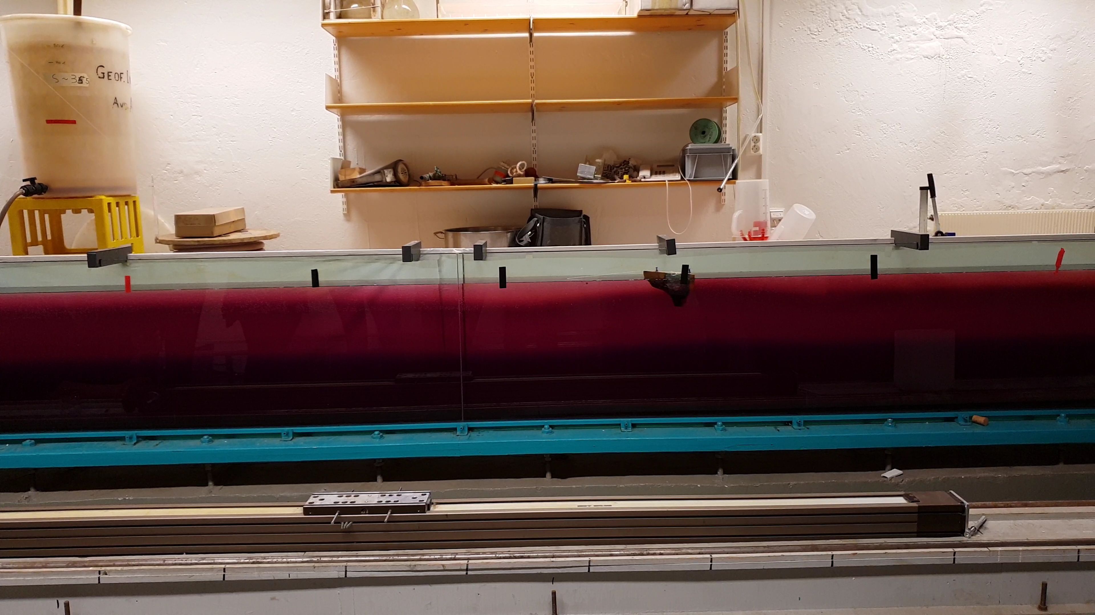
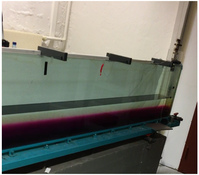
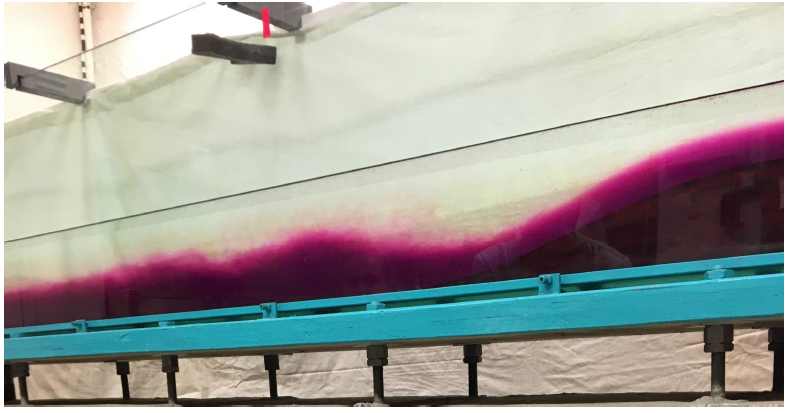
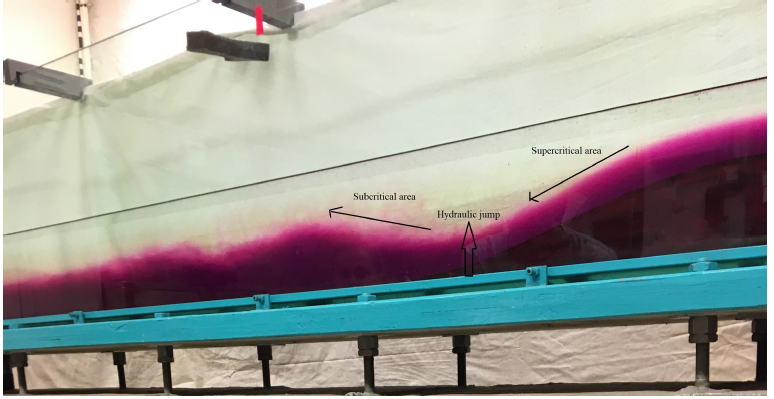
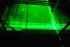
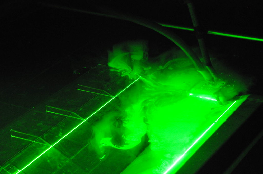
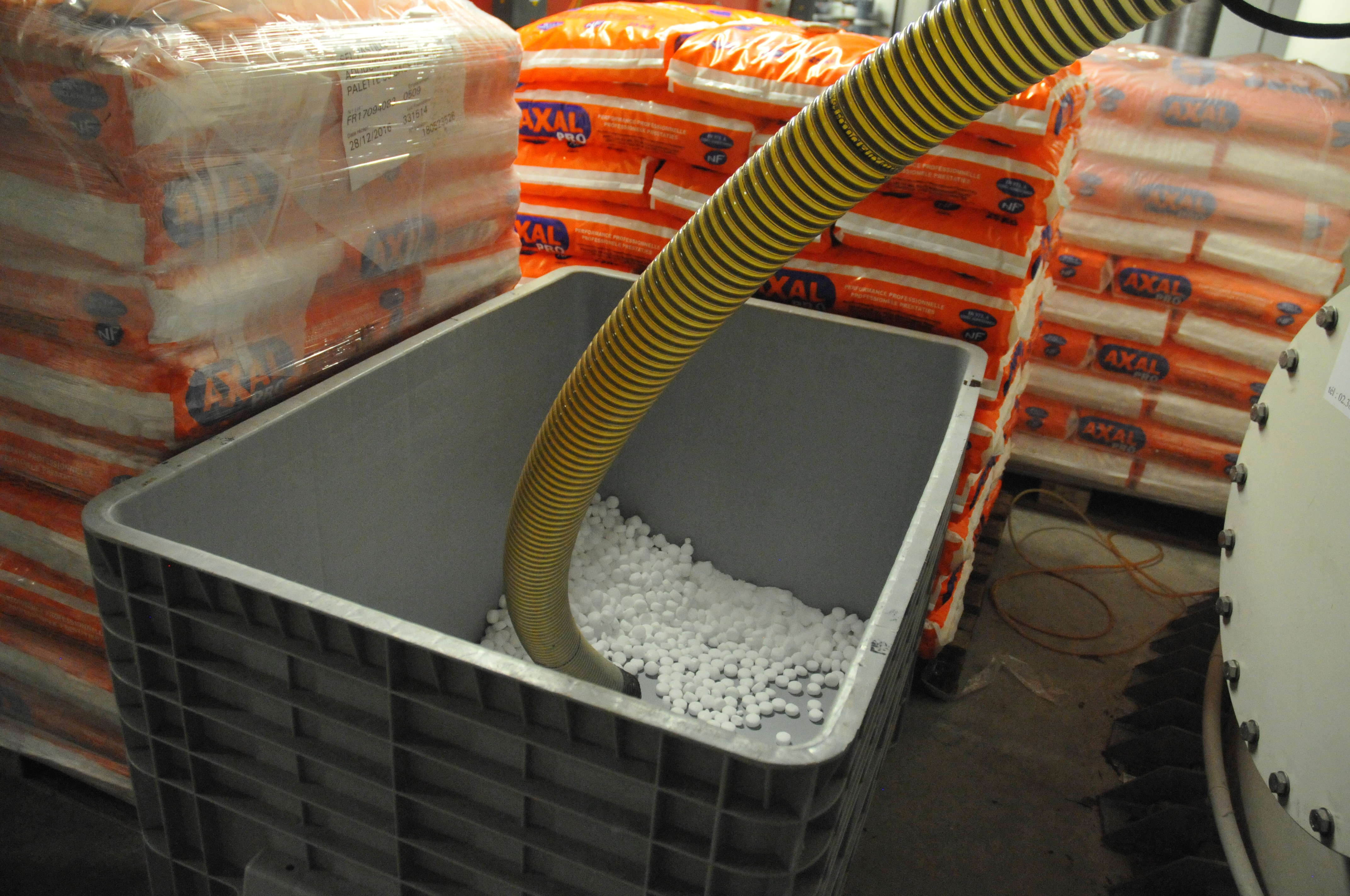
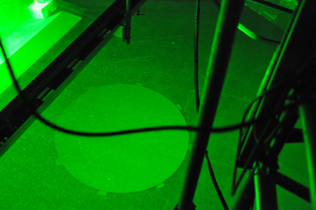
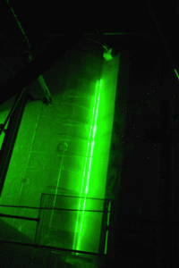
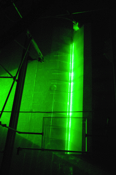
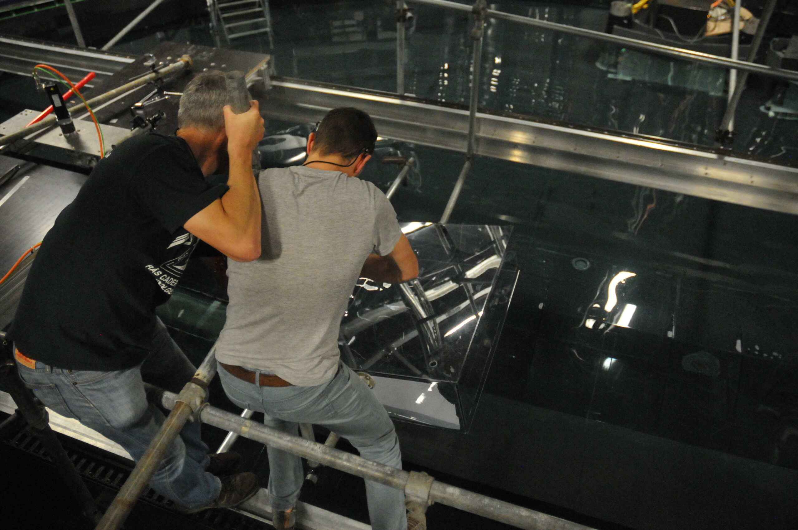
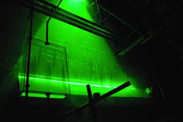
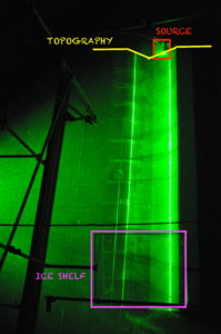
We performed an experiment (as seen in the video) where we recreated the ocean conditions and created an internal wave. Then we explored how and when the internal wave could influence the velocity of the ship. To simulate the conditions Nansen experienced, a wooden boat was pulled with constant force across a tank filled with water. The water had two layers, one fresh layer on top (clear), and one saline underneath (purple). The depth of the saline layer must be much greater than the depth of the fresh layer.

The experiment was performed several times with the boat being pulled with constant, but different, force. We expect that if the speed of the boat is larger than the speed of the internal wave, the boat will not feel the wave because it moves faster than the internal wave. If the speed of the boat is smaller than the speed of the internal wave (as seen in the video), the wave will catch up with the boat, and the speed of the boat will be much reduced.

Hydraulic jump

(by Cristina Arumi Planas, Elise Madeleine Colette Brunet, Haley Okun)

In order to observe Lee Waves and their related phenomenon, an experiment was conducted in a large water tank with a stratified two layer system. The two layer system was constructed with fresh water sitting atop colder salt water. The fresh water had a salinity of about 0‰, with a density of 1000 kg/m3 while the pink-dyed salt water had a salinity of about 35‰, and a density of 1028 kg/m3. In order to force Lee Waves to propagate, a mountain was moved along the bottom at two different speeds, fast and slow. While conducting an experiment to visualize Lee Waves, the phenomenon of the hydraulic jump can be observed. This event can be visualized when water flows over rocks or even in one’s kitchen sink. This occurs when water flowing over a surface goes from subcritical to supercritical, which is calculated through the Froude number. To calculate this, the velocity of the flow is divided by the phase speed of the shallow water gravity waves. The square root of this fraction is then taken to provide a unitless value called the Froude number. The result is either greater than one (supercritical) or less than one (subcritical). Supercritical Froude numbers indicate that waves cannot propagate upstream. This can physically be visualized when the flow over the observed surface goes from smooth and rather thin, to turbulent and rough. As we pushed the mountains through the stratified water, the denser saltwater (shown with pink dye) was forced up and over the mountain, resulting in turbulent motion just behind the surface anomaly. As the thinner flowing water moved from the downhill slope of the mountain to just downstream and onto the bottom of the tank, the flow went from smooth to rather chaotic. The interface where the flow becomes turbulent is the hydraulic jump. The smoother water flowing over the mountain is supercritical while the more mixed water just downstream is the subcritical flow. When the mountain was moved at the faster speed, this hydraulic jump was shifted accordingly. Instead of the hydraulic jump occurring just behind the mountain, the waves seemed to lag with the more turbulent flow occurring farther downstream than with the slower mountain speed.

Lee waves

(by: Jori Neteland-Kyte, Sara Elisabeth Holen Sælen , Susanne Moen Olsen)

Lee waves are a type of internal gravity waves, which is generated as fluid moves over an obstacle. The fluid needs to be stably stratified for this to occur. These waves can occur in both the atmosphere and in the ocean. (Cushman-Roisin and Beckers, 2011, page 412) To show this phenomenon it is convenient to perform a simple experiment, where a long tank is used. The tank is filled with stratified water, the bottom layer is denser than the layer above. A purple color is added to the denser water at the bottom layer, as seen in Figure 1.  This is done to distinguish between the two layers. The tank is also equipped with a moving obstacle which is possible to move at different constant velocities across the bottom of the tank.

Figure 1:The initial state of the two-layered stratified fluid.

When the obstacle is moved across the tank, waves are generated in the interface between the layers as seen in the figure 2.

Figure 2:Wave are generated when the obstacle is moved with the lowest speed.

Figure 3. displays how the Lee waves propagates, with the positions for the supercritical area, the hydraulic jump and subcritical area marked by the arrows. The supercritical area is positioned directly above the moving obstacle, which appears as one smooth wave. In the transition between the supercritical and the subcritical area, the hydraulic jump is found. This occurs at the end of the descending side of the moving obstacle. Following behind the
hydraulic jump is the subcritical area, this is where a train of waves are generated. These waves decays with time.

Figure 3: Position of sub- and super critical flow and the hydrualic jump.


Mesmerizing flow patterns and sad goodbyes

Written by Anna Wåhlin

It is the final day of experiments here at the Coriolis platform. The apartment is emptied of personal belongings, bicycles are being returned, goodbyes are stretched out. The lasers will soon be dark, the platform will grind to a halt and the tank will be emptied. It has been a fantastic time! I am amazed at what we have accomplished together during these weeks – answers to some of the most basic questions that are currently asked about the future for the Antarctic ice sheet.

Figure 2a-d: More mesmerizing flow patterns

The last days have been spent re-running some of the experiments that needed an extra quality-check, and we finished the very last one only an hour ago. Next week I will stay behind alone to try to get some nice photographs of the flow for our future publications. In order to prepare for that we were testing some different dyes. Red dye absorbs the light of the laser efficiently and gives a dark shadow on the images. Our all time favorite is Rhodamin – it is a fluorescent dye that produces its own light if you shine on it with green laser. We spent a good hour simply staring at the eddies and flow, mesmerized by the motion and flowing patterns. A very fine ending to the week! And a suitable finale to the time we have spent here on the rotating platform.

Video: Visualization of a beautiful barotropic eddy created outside the channel. It stayed like this for a good hour. You can see the barotropic structure since it moves in unison on the surface and below the surface, in a nearly perfect two-dimensional motion.

How salt changes the current

Until the beginning of the week we had only conducted barotropic experiments. This means that we induced fresh water into fresh water. How boring, you may thing… Well, although these experiments were very interesting, you are probably right because this setup doesn’t quite correspond to reality. At the coast of Antarctica, dense water is on one side produced by the growth of sea ice and on the other side origins from deep water that spills over the coast onto the continental shelf. Because the continental shelf slopes down towards the ice shelf, the dense water reaches towards the ice shelf. Our aim is to find out how the water behaves as it reaches the ice shelf front.

To reproduce this dense water flow, we inject salt enriched water into the channel. This relatively dense water approaches the ice shelf front along the left channel slope. To see a clear boundary between the dense and the fresh water, only a density difference of 1 kg/m3 is needed. The density difference increases the velocity of the current a lot, so that the experiments last much shorter. While the barotropic current was mainly blocked by the ice shelf front, the baroclinic current can freely enter the cavity beneath the ice shelf, as the dense water is largely decoupled from the freshwater. Because the fresh water layer above the dense current is barotropic, the previous experiments were of big interest as well to see how the upper layer behaves as the current reaches the ice shelf front.

On the cross section through the channel, the dense water separates clearly from the freshwater. It flows parallel to the slope to its left. Because we built a wall at the end of the channel (see our previous post: https://elindarelius.no/2017/10/20/closing-off-our-channel-at-the-ice-shelf-end-to-avoid-unrealistic-outflow/), the channel fills up quickly with salt water, which we have to evacuate after each experiment.

The dense, saline water contains many particles and gets visible in the vertical laser sheet. It flows towards the ice shelf (=towards us) along the slope to its left side.

In the photo of the cross section, you can also see 4 probes sticking in the water that we use to measure the density close to the source and close to the ice shelf front. We can then calculate the velocity of the dense current and the mixing between the fresh water and dense water along the channel.

In this experiment, we injected a flow that is 1kg/m3 denser than the ambient water. During the scans, the vertical laser shows the position of the dense current and the 4 probes (2 in front of the ice shelf front, 2 in front of the vertical laser) measure the change in density with time.

How to make sure the properties of water in a tank experiment are *just right*

For all our experiments here on the rotating platform in Grenoble, we have had a source, introducing an artificial current into our water-filled tank. With flow rates between 15 l/min and 60 l/min, and experiments running for about half an hour, that is a lot of water that has to come out of the source!

Below, you see a picture of the source during an experiment, and you see there is a pipe going into it, through which water is being supplied.

That water is coming from the very top of the rotating platform. There is a smaller tank up there which you see on the picture below. This is the tank where the particles which we use to visualize the flow field get added, and water in this tank needs to have the exact density we want our inflow to have. Not easy since it is sitting some 10 meters above the tank, where the air temperature is higher…

In fact, it’s an extremely complex system of tanks everywhere on and around the rotating platform. Below you see a picture of the screen through which most of them are operated:

There are three huuuuge water tanks in which water is prepared. You might have seen them rotating past in some of our videos, or you see them below (on the left you see the rotating tank). This picture doesn’t do them any justice: They are enormous. They are higher than the tank, and the mini tank on top of it, and the whole tent around all of it, and they start from the very bottom of the room (so not the level that seems to be the floor in the picture below).

We got to climb on one of them, which gave us a really great view of the tank (or at least that’s what Nadine says, and what the picture looks like — I was too busy getting over my fear of heights combined with the dizziness of a long working day on the rotating platform to enjoy it much ;-)).

Nadine has described earlier about how for some experiments, we add salt to spice things up. In the first set of experiments, for some, the whole tank was filled with salt water. And for this set of experiments, we sometimes added a small amount of salt to adjust the density of the inflow. But this is how producing the salt water actually works: Salt arrives in big bags, stacked on pallets. The salt pellets are put into the bin you see in the picture below, and get hoovered up into one of the huge tanks, where they are dissolved in water to make a saturated salt solution. That solution is then diluted to whatever salt concentration is desired for a certain experiment.

To fill a whole tank with salt water with approximately oceanic salinity, we need all the salt shown in the picture above!

We are pretty lucky that Thomas and Samuel take care of all the saltwater-making for us. That would be a huge task if we had to do it ourselves, and we are already now not getting bored 😉

And, btw, if you are wondering about how we are getting rid of the dense, salty current that we inject into the fresh ambient water in between experiments: The dense water eventually sinks to the bottom of the tank, slowly filling it up underneath the fresher water. You might have noticed those UFO-shaped flat plates on the bottom of the tank that you see in the picture below. They cover the outlets through which the tank can be drained, such that now water from the very bottom of the tank can be pumped out without introducing a vertical component (which would suck water from higher levels, too).

Quite a lot of effort going on not only to prepare the water, but also to get rid of it again! 🙂

And now on to even more realistic ice shelves!

We have already described experiments where our ice shelf was tilted, making the setup a little more realistic* than before (link here). But then later that day, we did two more experiments! And this time, the ice shelf wasn’t just tilted, it was also not going up all the way to the surface (or, well, it’s flat bottom did not, and then there was a sharp edge and the side of the ice shelf went out of the water). So we are expecting to see a mixture between the experiments shown is yesterday’s blog post: Some of the water being blocked by the ice shelf, but some possibly conserving its potential vorticity and going down the v of the canyon and then turning around and coming back up.

And that’s what we saw!

Can you spot the return flow that has come out from below the ice shelf in the lower layers before it gets obscured by all the stuff that got blocked by the ice shelf in the upper layers?

Nice when experiments really work out the way you expect them to do! 🙂

*I have a blogpost in the making on what “realistic” actually means in the context of geophysical fluid dynamics experiments, and if that is even something one should aim for (spoiler alert: not necessarily!), but I keep getting too distracted by all the cool stuff going on here in Grenoble, that it hasn’t progressed out of the draft stage. But I will finish it up and post it, I promise!

What happens when a current meets an obstacle? Topographic steering

As long as water depth and latitude stay the same, a current usually happily goes straight forward. However, a large part of what we are doing at the Coriolis tank in Grenoble has to do with what happens to ocean currents when they meet topography, so sea mounts, ridges or troughs under the water, and what happens then is called topographic steering.

Topographic steering basically means that a current will follow lines of constant potential vorticity (ω+f)/H. In this, ω is the rotation of the fluid (more on this here), f is the Coriolis parameter, and H is the water depth. So if a current is flowing  straight ahead (ω=0) in a sea of constant depth, it will stay at the one latitude where it started. If, however, there is a ridge or a canyon in its way, it will try to move such that it either changes its rotation or that it reaches a different latitude so that it stays on a path of constant (ω+f)/H.

What does that mean for our experiments?

In our experiments, we actually change the water depth not only by sloping the floor down into the canyon, we also change it by taking away height from the top by introducing ice shelves.

f in the tank is constant (explanation here), so only ω/H need to be conserved, meaning that the current needs to either follow lines of constant depth, or compensate for any depth change by changing its rotation. I have described in this post what that means for the flow in our tank: We expect — and observe visually (see picture on top of this post) — that an ice shelf that is tilted such that it is slowly decreasing the water depth will force the current down the slope of the canyon, until it reaches the deepest point, turns, and moves up again.

But now Nadine has plotted the actual measured data, and we see the same thing! Below you see a plot of the flow field on a level just below the upper edge of the canyon. I have drawn in where the ice shelf is situated and where the contours of the channel are, and, most importantly, that the flow field shows exactly the behaviour we were hoping for!


The messy flow field where the contours of the ice shelf are drawn in is probably because the data that is being plotted has been calculated from pictures that were taken from above the tank, through the ice shelf, so we don’t have good data in those spots. But all in all, we are very happy! And almost ready to call it a day. Almost ready, except it is still too exciting to think about our experiments… 😉

Tilting the ice shelf! Or: Our experiments are getting more realistic

Until now, we have used an “ice shelf” (a plastic box) which had a horizontal bottom (Read more about the general setup of the experiment in Nadine’s post). The bottom of the ice shelf was either right at the water’s surface, or lowered down into the water. What we see then is shown in the gif below, where we are scanning the full water depth from the bottom upward. The ice shelf is resting on the upper edge of the v-shaped channel, so it effectively blocks the flow, which separates at the ice edge and turns mainly left.

Now it’s time to get used to a new vantage point, which lets us look underneath the ice shelf. The source isn’t in the upper right-hand corner any more as it has been in all images and movies on this blog until now. See the sketch below: The source is in the upper right-hand corner and the ice shelf sits in the lower center of the picture, across the v-part of the channel.

The gif below shows the same experiment that we saw before, only this time from a similar perspective as shown in the sketch above: When the flow reaches the ice edge, it is blocked and turns to the side.

But then today, we have started tilting the ice shelf (well, Adrian and Thomas have, as you see in the image on top of this post, but I will keep saying “we”).

This might be more realistic — an ice shelf would probably have melted more the further out into the ocean you look (where the ice would have been exposed to melt longer and also the currents flowing under the ice shelf would still be warmer), and therefore we would expect the base of the ice shelf to slope up the further towards the open ocean you go. But this circulation is also one that is easier to understand theoretically: We are expecting the current to stay on lines of constant potential vorticity*. But it can only do that if those lines exist. In the previous experiments, there is a jump in potential vorticity introduced by the edge of the ice shelf, since the water depth decreases drastically as the current meets the ice shelf. Therefore there is no obvious way for the current to take since it can’t conserve its vorticity no matter where it goes (which is why we saw most of it just bouncing off the ice edge and flowing away to the sides). Now, we were hoping to see a circulation where the current, reaching the ice edge while it is flowing approximately half way down the slope, would be guided down the slope as the ice comes further and further down into the water, until at some point it crosses the deepest point of the slope, and turns backward, flowing up the slope and towards areas where the ice isn’t reaching as far down. That way, the water depth the current feels would always stay the same, since it is moving up and down the slope to compensate for the change in height introduced by the ice shelf.

So here is a gif of an experiment where the ice shelf is tilted such that its edge on the source-side is at water level, while the opposite edge rests on the edges of the canyon.

In case you can’t spot it, here is a sketch of the circulation:

So what I described above is actually exactly what we observed! Very very exciting! 🙂

*For a quick explanation of vorticity see this blog post — quick and dirty explanation is that if water depth changes, a water column will change its rotation. Either by moving to a place with a different planetary rotation (but it can’t do that in our tank, see here), or by starting to rotate itself and hence changing direction

First impression of the ice shelf experiments

This week we have started new experiments that use a V-shaped channel sloping down towards an ice shelf front. More than a whole week was used to remove the topography for the shelf break experiments and to build up a new topography, readjust the cameras and set up the lasers.

After some days of experiments, you will finally get to see some first time lapse videos of the current flowing towards the ice shelf! In these experiments, we want to find out how the current behaves as it reaches the ice shelf front. How much of the water gets blocked as it reaches the ice front that corresponds to a large step in water thickness? Does the water manage to flow underneath the ice shelf? In which direction does it go when it gets blocked? And what is happening inside the ice shelf cavity? As in the previous experiments, we are using a barotropic current (no density difference between the inflowing and the ambient water) and compare it to a baroclinic current (denser inflowing water than the ambient water).

With our GoPro that is installed high the topography in the center of the tank, we can record the current inside the channel. In this case, a barotropic current flows towards an ice shelf that is lowered 30 cm beneath the surface and sits on the wings of the V-shaped channel.

One of the cameras is installed on the left side of the above gif about 10m behind the ice shelf. It looks into the channel facing the source. With this camera, we are able to observe if the current is barotropic or not.

With the vertical laser sheet, we can see the cross section through the channel. The cloud of particles shows the location of the current, coming towards the camera. The transition between the current and the ambient water is very vertical, which shows that the flow is barotropic.

You may think that it sounds very easy to produce a barotropic flow – we just need to use the same water for the inflow as for the water inside the tank. But in reality it turns out that the current is very sensitive to small density differences and the inflowing water easily gets buoyant as it is stored under the roof of the rotating platform! However, a higher rotation speed seems to reduce the sensitivity to the density difference!