Topographic Rossby waves in a tank

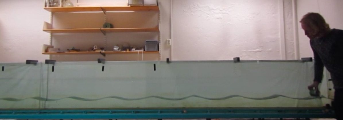
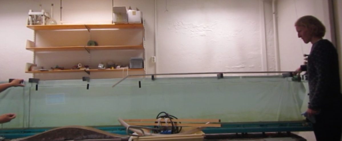
One experiment we wanted to run with the GEOF213 course this year were the Topographic Rossby Waves.

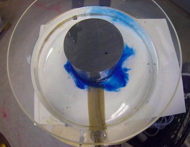
The idea is quite simple: We set a solid cylinder in the center of our tank and connect it with a ridge to the tank’s edge. The ridge is just a piece of hose that is taped radially to the bottom of the tank. We then spin the whole thing into solid body rotation. Once it is spun up, we add dye around the central cylinder. We then slow the tank down a tiny little bit, just enough so the water is moving relative to the tank and the ridge.

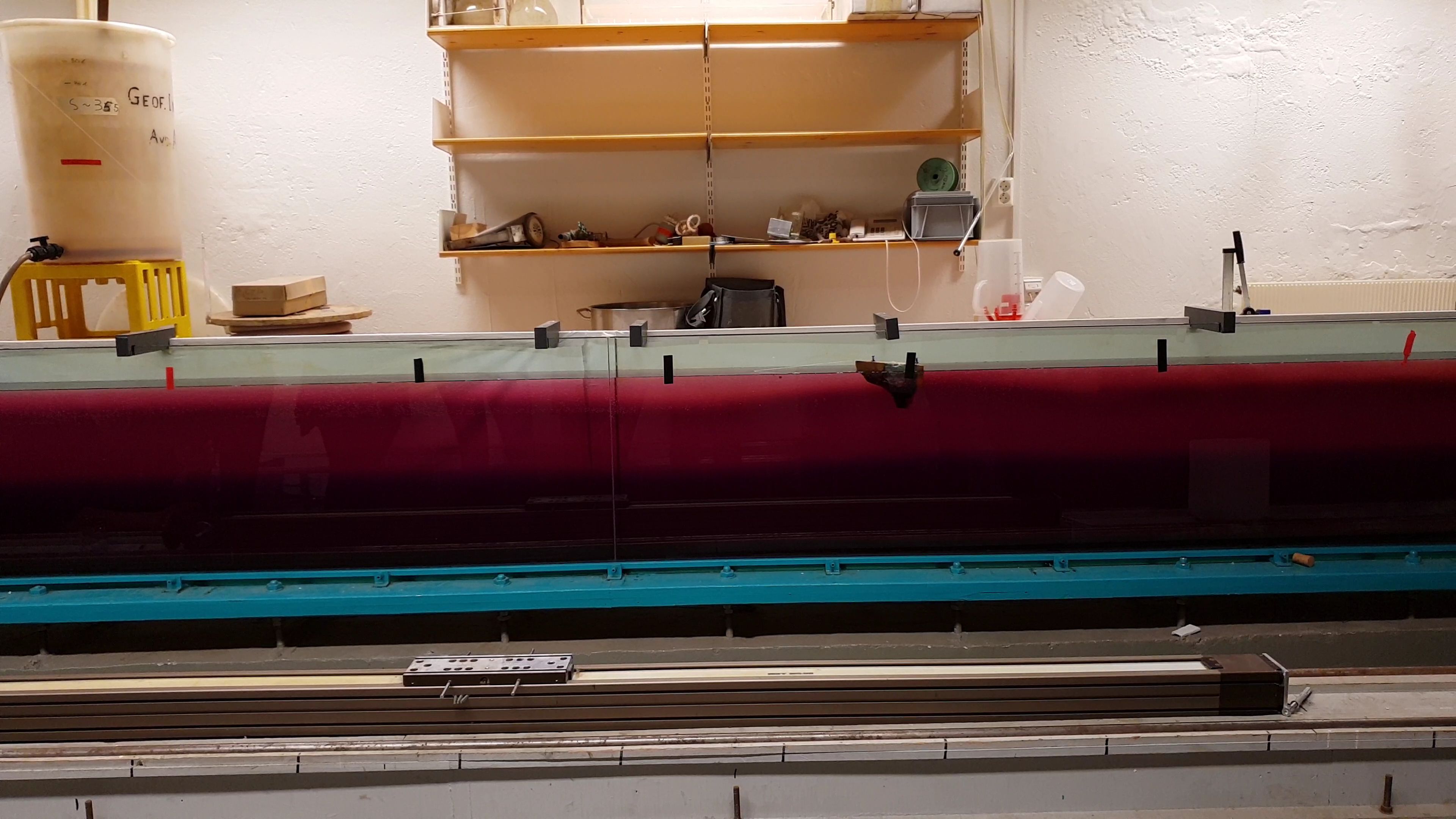
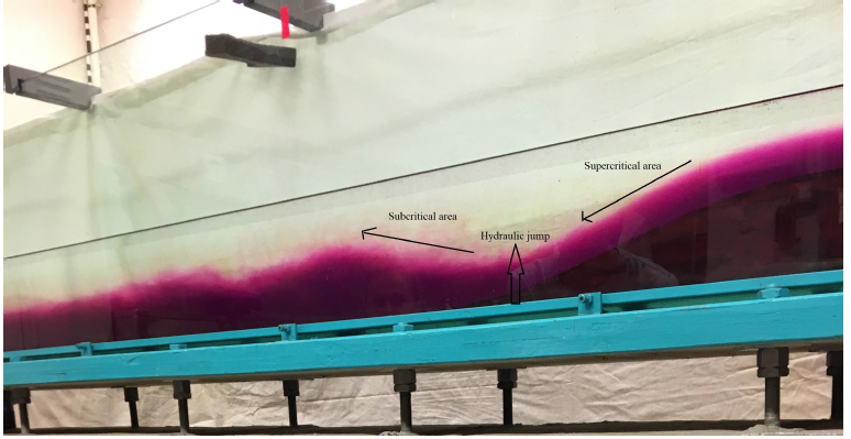
As the water now has to cross the ridge, it feels the water depth changing as it does so. A changing water depth results in changing relative vorticity to conserve potential vorticity, so the flow starts meandering.

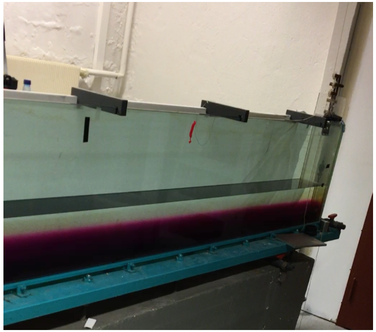
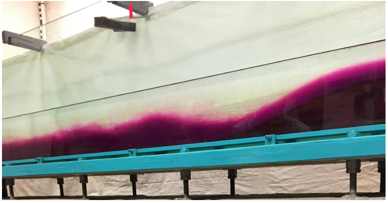
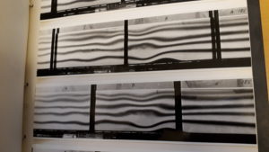
In both the picture above and below you see just that: Upstream of the ridge, the flow is (relatively) steady. But downstream of the ridge, topographic Rossby waves start developing.

In the end, we felt like the experiment was too difficult to run to rely on it working out when presenting it in class. But that doesn’t mean that I have given up on it. I will conquer the topographic Rossby waves eventually, so stay tuned! 🙂

Internal lee waves in a tank experiment

Another tank experiment that is run in GEOF213 this fall is the one where we are moving mountains. Or at least one mountain. Read last year’s students’ account of the experiment here!

We move the mountain through stagnant water in a tank in order to simulate the flow of water over a ridge. This creates internal waves in the “lee” of the mountain.

Watch the movie below to get an impression of how cool this looks! And don’t be confused by the split screen after the time lapse ends, I was trying to give you the best of both cameras at once…

Instructions for how to set up the experiment can be found here.

Explaining Nansen’s “dead water” observation with an experiment

When I (Mirjam) was visiting Elin at GFI last year, we set up Nansen’s “dead water” experiment in the 6m long tank in GFI’s basement to be used in GEOF213 to make things a little less theory-heavy and a little more easy to grasp. And since it’s about now that the experiment will be run again in GEOF213, I wanted to take the opportunity to remind you of how cool an experiment this is!

Out considerations for using this specific experiment in teaching are described here, including the learning outcomes we hope to achieve with the experiment. Students read original literature, determine the exact setup of the experiment, compare their theory-based predictions to actual observations. How much more fun can it get? Last year’s students even wrote a blog post about the experiment, which you can find here.

“Dead water”

In 1893, Nansen described a phenomenon he observed in the Arctic: “When caught in dead water Fram appeared to be held back, as if by some mysterious force, and she did not always answer the helm. In calm weather, with a light cargo, Fram was capable of 6 to 7 knots. When in dead water she was unable to make 1.5 knots. We made loops in our course, turned sometimes right around, tried all sorts of antics to get clear of it, but to very little purpose.” (cited in Walker,  J.M.; “Farthest North, Dead Water and the Ekman Spiral,” Weather, 46:158, 1991)

The experiment we set up shows the mechanism that explains Nansen’s observation. Energy from the propulsion of the ship is used to generate internal waves at the interface between a shallow, fresh surface layer and the denser, more salty deep layer below. If the ship is moving slowly enough that the internal wave it generates has the chance to catch up with the ship, an interaction between the internal wave and ship will take place. This will slow down the ship much the same way that Nansen described.

Instructions for how to set up that experiment can be found here.

Looking at the phase velocities of shallow water and deep water waves in an experiment

Calculating the phase velocities of shallow water and deep water waves from the dispersion relation sometimes seems a bit pointless to students (at least it sure did to me (Mirjam) when I had to do it during my studies years ago). So Elin and I played around with it a bit (thanks to a suggestion by Tor Gammelsrød, who always comes to visit us in the lab!), and now there is a new experiment included in GEOF213 to complement the theoretical exercises that were already in place.

Look at Elin exciting shallow water waves in the picture below. It’s quite easy to imagine how one could measure the waves’ phase speed in the lab, just by taking the time it takes for them to run over a known distance, right? (Btw, this is the shallow water experiment that is part of the 2nd-year instruction, so students should already be familiar with shallow water waves)

Things get a little more complicated if there is more water in the tank, as you see in the picture below. Not only do waves have a smaller amplitude (because we didn’t want to risk flooding the lab), but also there is the thing about phase velocity and group velocity in deep water, that makes both of them a lot harder to observe! We don’t want any spoilers here, but you know what I am talking about…

This is such a simple experiment to run, but having the 6m long tank really helps because it gives us at least some time to observe waves before the reflections from the far end come back to haunt us.

And it is quite difficult to excite waves with more or less constant wave lengths. “Allegro!” is what Elin gave me as instructions for what kind of waves she wanted. Playing with a tank with Elin is always the best!

Sometimes you have to see it to believe it — or to wanting to be able calculate it. Planetary Rossby waves in a tank!

In the image above, we see planetary Rossby waves. They are propagating along the slope with shallow water to the right. But why? This is the kind of thing one might learn in GEOF213: “Dynamics of Ocean and Atmosphere”. This is theoretical subject, with equations filling the blackboard in most of the classes. To make it more fun, to help understanding of mechanisms and to motivate why a little theory really can’t be avoided, Elin and I (Mirjam) set up a couple of experiments over the last couple of weeks. Some working better than others, but that was to be expected…

But one that worked super well are planetary Rossby waves. We use a square tank with a sloping bottom which is spun up to solid body rotation. Then, a colored ice cube is placed in the shallow eastern corner of the tank. As it starts melting, a column of melt water forms below it. Because the melt water column is being stretched as it is sinking, it starts spinning. Once it reaches the sloping bottom, it is stretched even further. In order to conserve potential vorticity, it moves back up the slope again, starting to form a Rossby wave which then propagates westward.

Below you see an experiment both from the top (upper left corner) and the side.

What I find super cool is that the ice cube, sitting on top of its rotating Taylor column, spins in the same direction as the tank, but even faster than the tank itself! Physics says it has to, of course, but this is the kind of counterintuitive stuff that is just really nice to directly observe.

Here is another experiment, shown in real time.

Dead water

 (by: Torunn Sandven Sagen, Petter Ekrem, Eirik Nordgård)

In 1893, during the Fram expedition, Fridtjof Nansen and his crew encountered a phenomenon where the velocity of the ship was reduced significantly, even though the engine was working at full speed. Nansen described this phenomenon as “dead water” (Brady, 2014). This dead water effect can happen when the ship creates an internal wave as it moves through water. The water must be stratified, meaning that the top layer is less dense than the bottom layer. At the same time, the draught of the ship must have the same depth as the top layer. The internal wave produces a drag, reducing the velocity of the ship. The speed of the wave is only dependent of densities and depth of the layers, not the velocity of the ship. (Grue, 2018).

We performed an experiment (as seen in the video) where we recreated the ocean conditions and created an internal wave. Then we explored how and when the internal wave could influence the velocity of the ship. To simulate the conditions Nansen experienced, a wooden boat was pulled with constant force across a tank filled with water. The water had two layers, one fresh layer on top (clear), and one saline underneath (purple). The depth of the saline layer must be much greater than the depth of the fresh layer.

The experiment was performed several times with the boat being pulled with constant, but different, force. We expect that if the speed of the boat is larger than the speed of the internal wave, the boat will not feel the wave because it moves faster than the internal wave. If the speed of the boat is smaller than the speed of the internal wave (as seen in the video), the wave will catch up with the boat, and the speed of the boat will be much reduced.

Hydraulic jump

(by Cristina Arumi Planas, Elise Madeleine Colette Brunet, Haley Okun)

In order to observe Lee Waves and their related phenomenon, an experiment was conducted in a large water tank with a stratified two layer system. The two layer system was constructed with fresh water sitting atop colder salt water. The fresh water had a salinity of about 0‰, with a density of 1000 kg/m3 while the pink-dyed salt water had a salinity of about 35‰, and a density of 1028 kg/m3. In order to force Lee Waves to propagate, a mountain was moved along the bottom at two different speeds, fast and slow. While conducting an experiment to visualize Lee Waves, the phenomenon of the hydraulic jump can be observed. This event can be visualized when water flows over rocks or even in one’s kitchen sink. This occurs when water flowing over a surface goes from subcritical to supercritical, which is calculated through the Froude number. To calculate this, the velocity of the flow is divided by the phase speed of the shallow water gravity waves. The square root of this fraction is then taken to provide a unitless value called the Froude number. The result is either greater than one (supercritical) or less than one (subcritical). Supercritical Froude numbers indicate that waves cannot propagate upstream. This can physically be visualized when the flow over the observed surface goes from smooth and rather thin, to turbulent and rough. As we pushed the mountains through the stratified water, the denser saltwater (shown with pink dye) was forced up and over the mountain, resulting in turbulent motion just behind the surface anomaly. As the thinner flowing water moved from the downhill slope of the mountain to just downstream and onto the bottom of the tank, the flow went from smooth to rather chaotic. The interface where the flow becomes turbulent is the hydraulic jump. The smoother water flowing over the mountain is supercritical while the more mixed water just downstream is the subcritical flow. When the mountain was moved at the faster speed, this hydraulic jump was shifted accordingly. Instead of the hydraulic jump occurring just behind the mountain, the waves seemed to lag with the more turbulent flow occurring farther downstream than with the slower mountain speed.

Lee waves

(by: Jori Neteland-Kyte, Sara Elisabeth Holen Sælen , Susanne Moen Olsen)

Lee waves are a type of internal gravity waves, which is generated as fluid moves over an obstacle. The fluid needs to be stably stratified for this to occur. These waves can occur in both the atmosphere and in the ocean. (Cushman-Roisin and Beckers, 2011, page 412) To show this phenomenon it is convenient to perform a simple experiment, where a long tank is used. The tank is filled with stratified water, the bottom layer is denser than the layer above. A purple color is added to the denser water at the bottom layer, as seen in Figure 1.  This is done to distinguish between the two layers. The tank is also equipped with a moving obstacle which is possible to move at different constant velocities across the bottom of the tank.

Figure 1:The initial state of the two-layered stratified fluid.

When the obstacle is moved across the tank, waves are generated in the interface between the layers as seen in the figure 2.

Figure 2:Wave are generated when the obstacle is moved with the lowest speed.

Figure 3. displays how the Lee waves propagates, with the positions for the supercritical area, the hydraulic jump and subcritical area marked by the arrows. The supercritical area is positioned directly above the moving obstacle, which appears as one smooth wave. In the transition between the supercritical and the subcritical area, the hydraulic jump is found. This occurs at the end of the descending side of the moving obstacle. Following behind the
hydraulic jump is the subcritical area, this is where a train of waves are generated. These waves decays with time.

Figure 3: Position of sub- and super critical flow and the hydrualic jump.


Long time no seen…

There hasn’t been much happening on this blog lately, since I’ve been busy, busy, busy teaching geophysical fluid dynamics to the third year bachelor students here at GFI. My job description as an associate professor at UiB includes 50% teaching – however giving the (somewhat equation heavy) course for the first time it felt more like 150%… but now the last lecture is given, the students are happily (?) preparing for the exam, and I finally have time to do some science… and to update the blog!

First I’ll have the students tell and show you what they did with Mirjam when she was visiting the Bjerknes centre and Bergen in October. One flight of stairs down from my office, in the basement of GFI, there is a 6 m long tank. It is not round and it is not rotating (like the tank in Grenoble), but it can move mountains! Or rather, it holds a mountain that can be moved. Why would one want to move a mountain in a tank? Well, as Arne Foldvik, the professor emiritus who built the tank a few decades ago realized, if you want to study flow over topography in the lab, then it is easier to have the fluid move beneath the fluid than to make the fluid move over the mountain… and the physics are the same.

Arne (who later left the lab and became on of the Norwegian pioneers in Antarctic oceanography) spent years with the tank – my student only spent an hour but they did some really nice stuff! Thank you again Mirjam for setting it all up – and thanks to the students for handing in the (non-compluslory) assignments that you’ll be able to read (and watch) in the days to come!

Below you see Arne Foldvik showing off his results – and inspecting his old tank.

Arne Foldvik inspecting his tank
All Arne’s experiments were documented by GFI’s in house (!) photographer!
Detailed logbooks…